Cell type abundance analysis in scRNA-seq
By clustering, thresholds based on marker genes, or label transfer, cells in single-cell RNA-seq data can be assigned cell type labels. One use of scRNA-seq data is to compare abundance of cell types between experimental conditions or tissues. If a cell type is enriched in a disease condition it is an interesting avenue to explore what causes this increase in abundance.
Generalized linear models give a very simple yet powerful framework to study differences in cell type abundance. Each cell type can be considered to be sampled from a population of cells in an experimental sample.
Using a binomial linear model one can analyse counts of repeated observations of binary choices.
$$ N_{\text{cell type in sample}} \sim \text{B}(p, N_{\text{total cells in sample}}) $$ $$ \text{logit}(p) = \beta X $$
There are a large number of packages that can analyze this kind of model. They all differ slightly in how to provide values. The glm package in R takes these counts as paired observations of the form \( (N_{\text{cell type in sample}}, N_{\text{other cells in sample}}) = (N_{\text{cell type in sample}}, N_{\text{total cells in sample}} - N_{\text{cell type in sample}}) \).
To illustrate how a binomial GLM can be used to analyze cell type count data we use data from Smillie et al. Here the authors have 51 cell types (‘Cluster’) from a total of 365,492 cells from a number of individuals in healthy, non-inflamed, and inflamed states of ulcerative colitis. How can we analyze which cell types are enriched in inflamed samples?
By taking the metadata of the cells published with the paper, we can group the samples and count how many of each cell type are in each sample. For the input to the binomial GLM, we also calculate the total number of cells in each sample, and create an ‘Other’ column which have the number of cells in the sample not from the cell type of interest.
   Health  batch Location Subject Cluster               Count Total Other
   <chr>   <chr> <chr>    <chr>   <chr>                 <dbl> <dbl> <dbl>
 1 Healthy 0     Epi      N8      Best4+ Enterocytes       21   932   911
 2 Healthy 0     Epi      N8      CD4+ Activated Fos-hi     0   932   932
 3 Healthy 0     Epi      N8      CD4+ Activated Fos-lo     0   932   932
 4 Healthy 0     Epi      N8      CD4+ Memory               0   932   932
 5 Healthy 0     Epi      N8      CD4+ PD1+                 0   932   932
 6 Healthy 0     Epi      N8      CD8+ IELs                 0   932   932
 7 Healthy 0     Epi      N8      CD8+ IL17+                0   932   932
 8 Healthy 0     Epi      N8      CD8+ LP                   0   932   932
 9 Healthy 0     Epi      N8      CD69+ Mast                0   932   932
10 Healthy 0     Epi      N8      CD69- Mast                0   932   932
As a warmup, let us use a GLM to estimate the proportions of the cell types across all the samples, treating the samples as replicates. In this case a simple model can be made where Count vs Other only depends on the cell type identity
model0 <- glm(
  formula = cbind(Count, Other) ~ Cluster,
  family = binomial(link = 'logit'),
  data = df_a
)
An extremely useful tool when working with GLMs is the emmeans package. This package can transform a parameterization of a linear model to return any mean or contrast that is of interest. From the data and the simple linear model, we can obtain per-cell-type probability values with emmeans
emm0 <- emmeans(model0, specs = ~ Cluster)
emm0 %>%
summary(infer = TRUE, type = 'response') %>%
arrange(prob) -> cell_type_probs
cell_type_probs %>% head
Cluster prob SE df asymp.LCL asymp.UCL z.ratio p.value
1 CD69- Mast 0.0003912534 3.271185e-05 Inf 0.0003321153 0.0004609172 -93.80333 0
2 Cycling Monocytes 0.0009576133 5.116207e-05 Inf 0.0008624047 0.0010633216 -129.96235 0
3 RSPO3+ 0.0009904458 5.203089e-05 Inf 0.0008935369 0.0010978534 -131.52763 0
4 CD4+ PD1+ 0.0011409278 5.583960e-05 Inf 0.0010365643 0.0012557858 -138.26581 0
5 DC1 0.0011710243 5.657044e-05 Inf 0.0010652300 0.0012873120 -139.53652 0
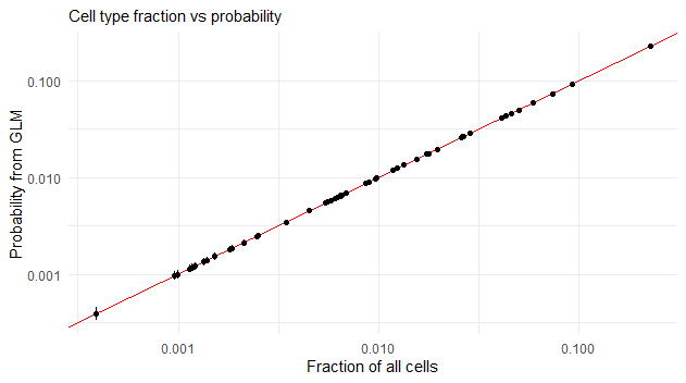
6 M cells 0.0012065928 5.742212e-05 Inf 0.0010991312 0.0013245468 -141.00855 0The results can be compared with a much simpler strategy to get the cell type proportions: counting the cells per cell type in the data and dividing by the total number of cells.
df_a %>% pull(Count) %>% sum -> N
df_a %>%
  group_by(Cluster) %>%
  summarise(fraction = sum(Count) / N) %>%
  arrange(fraction) %>%
  as.data.frame -> cell_type_fractions

cell_type_fractions %>% left_join(cell_type_probs) -> cell_type_probs
So why bother with the GLM? Because with the GLM we can make predictors for cell type proportions that depend on predictors of interest (inflamed vs healthy), as well as accounting for batch effects and making use of replicates.
The ‘Health’ variable in the data contains ‘Healthy’, ‘Non-inflamed’ and ‘Inflamed’. For the sake of simplicity we will just consider ‘Healthy’ and ‘Inflamed’ here, so filter out ‘Non-inflamed’ samples.
We want to compare ‘Healthy’ and ‘Inflamed’ while accounting for variation due to ‘Location’ and ‘batch’. We do this by making a more complicated linear model
df_a %>% filter(Health %in% c('Healthy', 'Inflamed')) -> df
formula = cbind(Count, Other) ~ Cluster * Health + Cluster * Location + Cluster * batch
model1 <- glm(formula = formula, family = 'binomial', data = df)
Here the abundance of a given cell type depends on whether ‘Health’ is ‘Inflamed’ or ‘Healthy’. In addition, the abundance of the same cell type depends on ‘location’ and ‘batch’. After fitting the model we can compare odds ratios of ‘Inflamed’ vs ‘Healthy’ for each ‘Cluster’ using emmeans.
emm1 <- emmeans(model1, specs = revpairwise ~ Health | Cluster)
emm1$contrasts %>%
summary(infer = TRUE, type = 'response') %>%
rbind() %>%
as.data.frame() -> c_results
contrast Cluster odds.ratio SE df asymp.LCL asymp.UCL z.ratio p.value
1 Inflamed / Healthy Inflammatory Fibroblasts 62.4847804 14.10944910 Inf 40.1391051 97.2704243 18.31182457 6.660029e-75
2 Inflamed / Healthy M cells 16.5045991 3.48168172 Inf 10.9154622 24.9555893 13.29039892 2.631714e-40
3 Inflamed / Healthy Inflammatory Monocytes 4.1921875 0.40353981 Inf 3.4713953 5.0626433 14.88908404 3.880492e-50
4 Inflamed / Healthy Pericytes 4.1163273 0.50315305 Inf 3.2393999 5.2306448 11.57588915 5.460220e-31
5 Inflamed / Healthy Post-capillary Venules 3.1448881 0.19793669 Inf 2.7799134 3.5577803 18.20453090 4.751058e-74
6 Inflamed / Healthy Cycling B 2.5302852 0.15369320 Inf 2.2462922 2.8501826 15.28333532 9.875431e-53
7 Inflamed / Healthy GC 2.3807061 0.21261039 Inf 1.9984290 2.8361086 9.71268497 2.662299e-22
8 Inflamed / Healthy Endothelial 2.1209671 0.12396363 Inf 1.8914025 2.3783945 12.86422519 7.155584e-38
9 Inflamed / Healthy CD4+ PD1+ 1.9756741 0.25707939 Inf 1.5309286 2.5496212 5.23284107 1.669243e-07
10 Inflamed / Healthy Follicular 1.9259575 0.03832100 Inf 1.8522954 2.0025490 32.94061154 5.765493e-238
11 Inflamed / Healthy Myofibroblasts 1.8911035 0.12724192 Inf 1.6574584 2.1576845 9.46964966 2.807838e-21
12 Inflamed / Healthy Enteroendocrine 1.7511544 0.23462541 Inf 1.3467211 2.2770429 4.18168012 2.893629e-05
13 Inflamed / Healthy Tregs 1.6836653 0.06086953 Inf 1.5684919 1.8072958 14.41023630 4.461813e-47
14 Inflamed / Healthy Tuft 1.6445042 0.15265295 Inf 1.3709489 1.9726441 5.35882535 8.376478e-08
15 Inflamed / Healthy Enterocytes 1.6271677 0.06957659 Inf 1.4963580 1.7694126 11.38560877 4.932258e-30
16 Inflamed / Healthy CD69+ Mast 1.5857281 0.06127444 Inf 1.4700675 1.7104885 11.93140033 8.119601e-33
17 Inflamed / Healthy CD4+ Memory 1.4140279 0.02517604 Inf 1.3655348 1.4642431 19.45814530 2.486205e-84
18 Inflamed / Healthy Goblet 1.3441453 0.08543563 Inf 1.1867049 1.5224733 4.65311890 3.269516e-06
19 Inflamed / Healthy CD8+ IL17+ 1.2856555 0.15437166 Inf 1.0160588 1.6267858 2.09264426 3.638092e-02
20 Inflamed / Healthy Immature Goblet 1.2676903 0.04573710 Inf 1.1811433 1.3605789 6.57435120 4.886577e-11
21 Inflamed / Healthy Best4+ Enterocytes 1.1589660 0.06670085 Inf 1.0353384 1.2973557 2.56338886 1.036559e-02
22 Inflamed / Healthy Stem 1.1518704 0.07809549 Inf 1.0085400 1.3155704 2.08538999 3.703391e-02
23 Inflamed / Healthy Macrophages 1.1339316 0.02410242 Inf 1.0876623 1.1821693 5.91330273 3.353151e-09
24 Inflamed / Healthy TA 1 1.0774633 0.02269981 Inf 1.0338785 1.1228854 3.54139389 3.980189e-04
25 Inflamed / Healthy Cycling TA 1.0770687 0.02800200 Inf 1.0235606 1.1333739 2.85568871 4.294359e-03
26 Inflamed / Healthy Cycling T 1.0412753 0.10986760 Inf 0.8467459 1.2804953 0.38333047 7.014748e-01
27 Inflamed / Healthy WNT2B+ Fos-lo 2 1.0233590 0.05237077 Inf 0.9256941 1.1313281 0.45120147 6.518444e-01
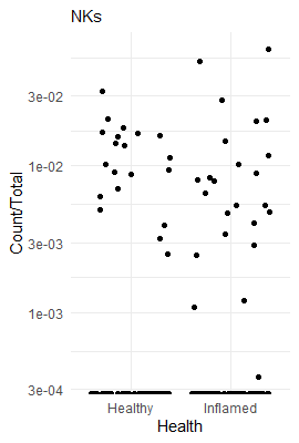
28 Inflamed / Healthy NKs 0.9952119 0.05914589 Inf 0.8857849 1.1181571 -0.08076013 9.356327e-01
29 Inflamed / Healthy TA 2 0.9930944 0.02931542 Inf 0.9372677 1.0522462 -0.23474820 8.144042e-01
30 Inflamed / Healthy Secretory TA 0.9134756 0.04545739 Inf 0.8285878 1.0070602 -1.81858714 6.897444e-02
31 Inflamed / Healthy CD8+ LP 0.8908214 0.01948936 Inf 0.8534303 0.9298506 -5.28437421 1.261352e-07
32 Inflamed / Healthy Plasma 0.8881827 0.01002867 Inf 0.8687427 0.9080576 -10.50176601 8.477899e-26
33 Inflamed / Healthy Immature Enterocytes 2 0.8734444 0.03039523 Inf 0.8158571 0.9350966 -3.88832100 1.009401e-04
34 Inflamed / Healthy ILCs 0.6891946 0.07523673 Inf 0.5564414 0.8536194 -3.40977118 6.501740e-04
35 Inflamed / Healthy DC1 0.6608477 0.07781771 Inf 0.5246488 0.8324038 -3.51776226 4.352021e-04
36 Inflamed / Healthy Immature Enterocytes 1 0.6592190 0.02539055 Inf 0.6112864 0.7109101 -10.81883637 2.803136e-27
37 Inflamed / Healthy WNT2B+ Fos-hi 0.6524180 0.02751867 Inf 0.6006516 0.7086457 -10.12505367 4.277440e-24
38 Inflamed / Healthy DC2 0.5976786 0.03078289 Inf 0.5402905 0.6611622 -9.99342232 1.628598e-23
39 Inflamed / Healthy WNT5B+ 1 0.5906783 0.03069201 Inf 0.5334849 0.6540034 -10.13235991 3.969516e-24
40 Inflamed / Healthy WNT5B+ 2 0.5801389 0.02750838 Inf 0.5286530 0.6366391 -11.48299320 1.606219e-30
41 Inflamed / Healthy WNT2B+ Fos-lo 1 0.5559970 0.02165505 Inf 0.5151334 0.6001021 -15.07112820 2.507935e-51
42 Inflamed / Healthy Enterocyte Progenitors 0.4850947 0.01928310 Inf 0.4487353 0.5244001 -18.19846809 5.307127e-74
43 Inflamed / Healthy CD4+ Activated Fos-hi 0.4497154 0.01155000 Inf 0.4276382 0.4729325 -31.11565882 1.479043e-212
44 Inflamed / Healthy CD4+ Activated Fos-lo 0.4256359 0.01102951 Inf 0.4045582 0.4478117 -32.96301722 2.753587e-238
45 Inflamed / Healthy Microvascular 0.3241644 0.03439802 Inf 0.2632946 0.3991065 -10.61609664 2.508316e-26
46 Inflamed / Healthy RSPO3+ 0.3030192 0.04640930 Inf 0.2244415 0.4091071 -7.79569031 6.405731e-15
47 Inflamed / Healthy Glia 0.2698563 0.02237938 Inf 0.2293727 0.3174851 -15.79469705 3.384151e-56
48 Inflamed / Healthy CD69- Mast 0.2300449 0.05171148 Inf 0.1480717 0.3573988 -6.53716643 6.269527e-11
49 Inflamed / Healthy Cycling Monocytes 0.2278063 0.03064635 Inf 0.1750069 0.2965352 -10.99591380 3.998428e-28
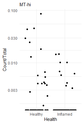
50 Inflamed / Healthy MT-hi 0.2235797 0.02702011 Inf 0.1764261 0.2833362 -12.39519687 2.774635e-35
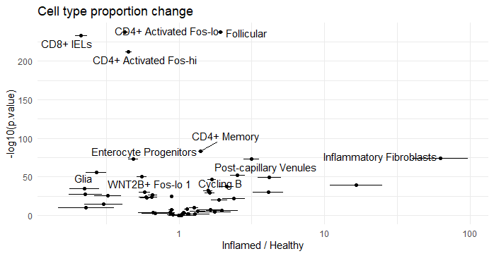
51 Inflamed / Healthy CD8+ IELs 0.2130551 0.01009845 Inf 0.1941540 0.2337962 -32.62151756 2.031799e-233We see that the most enriched cell types are ‘Inflammatory Fibroblasts’, ‘M cells’, and ‘Inflammatory Monocytes’. The results from emmeans are in the unit of odds ratios. ‘Inflammatory Fibroblasts’ have an odds ratio of 62.5, which means the odds of seeing an ‘Inflammatory Fibroblast’ in an ‘Inflamed’ sample is 62.5 times higher than seeing an ‘Inflammatory Fibroblast’ in a healthy sample.These results can be visualized as a volcano plot to compare statistical significance and odds ratio for each cell type.
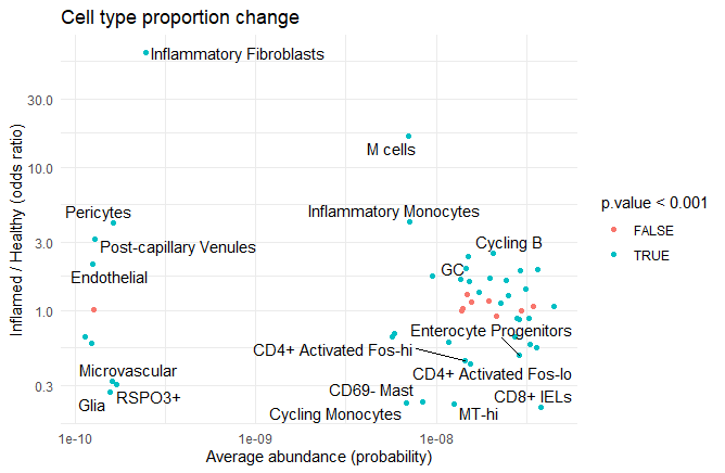
We can also extract the mean abundance for each ‘Cluster’ from the model using emmeans with a different ‘specs’ parameter. After putting this together with the previous results we can make an MA-plot to relate odds ratio with the average abundance of each cell type.
emm2 <- emmeans(model1, specs = ~ Cluster)
emm2 %>%
  summary(type = 'response') %>%
  select(Cluster, prob) -> mean_probs

c_results %>% left_join(mean_probs) -> m_results
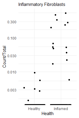
To see how enriched looks in the raw data, we can plot a couple of cell types as a fraction of all cells in a sample. This way we can illustrate how a highly enriched cell type looks, compared to a non-enriched cell type, compared to a highly depleted cell type.
Generalized linear models are great tools to analyse various observed counts and known conditions. The largest inconvenience with GLMs is keeping track of parameter names, and transforming parameters to create contrasts to answer questions. The emmeans package really supercharges analysis using GLMS by tracking variable names and transformations for you.
An R file and data for this analysis are available at Github.