The scVI package provides a conditional variational autoencoder for the integration and analysis of scRNA-seq data. This is a generative model that uses a latent representation of cells which can produce gene UMI counts which have similar statistical properties as the observed data. To effectively use scVI it is best to think of it in terms of the generative model rather than the “auto encoder” aspect of it. That the latent representation is inferred using amortized inference rather than any other inference algorithm is more of an implementation detail.

This post goes through step by step how scVI takes the cell representation and is able to generate scRNA-seq UMI counts.

In summary, the steps are:

\[ W = f(Z, c) \] \[ X = g(W), \] \[ \omega = softmax(X), \] \[ \Lambda = \omega * \ell, \] \[ Y \sim NB(\Lambda, \theta), \]

A very good example dataset is one by Hrvatin et al. This data consists of UMI counts for 25,187 genes from 48,266 cells, sampled from the visual cortex of 28 mice (in three experimental conditions).

To illustrate the generative process in scVI, each step will use three genes (where applicable) to illustrate how each step goes towards generating counts. These are: Slc17a7, a marker for excitatory neurons; Olig1, a marker for oligodendrocytes; and Nr4a2, a gene which activates expression in some cell types when the mice are receiving light stimulation. It is clear that these genes have heterogeneity beyond observational noise, which makes them good candidates for illustration.

Below are three histograms of the observed UMI counts of these genes. The x-axis shows UMI counts between 1 and 25 for the gene, and the y-axis shows how many cells in the raw data that number of UMI counts is observed in.

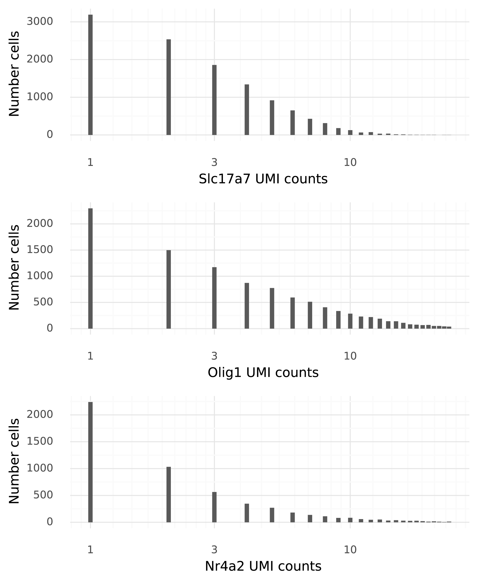
After the data generative process has completed, the goal is to obtain data with very similar histograms to these.

\( Z \in \mathbb{R}^{10} \)

The journey towards generating counts starts with the representation \( Z \). Each cell is represented by a 10-dimensional vector \( z_i \) which describes the structured heterogeneity in the data. The goal is that cells that are close together in this representation have similar transcriptomes. A nice thing with scVI is that it estimates a posterior distribution for each \( z_i \), but in this post the focus is on the mean of \( z_i \). It is not feasible to visualize the 10-dimensional representation of the data, but we can create a tSNE visualization of the \( Z \), and color it by information that was provided in the published dataset from Hrvatin et al.

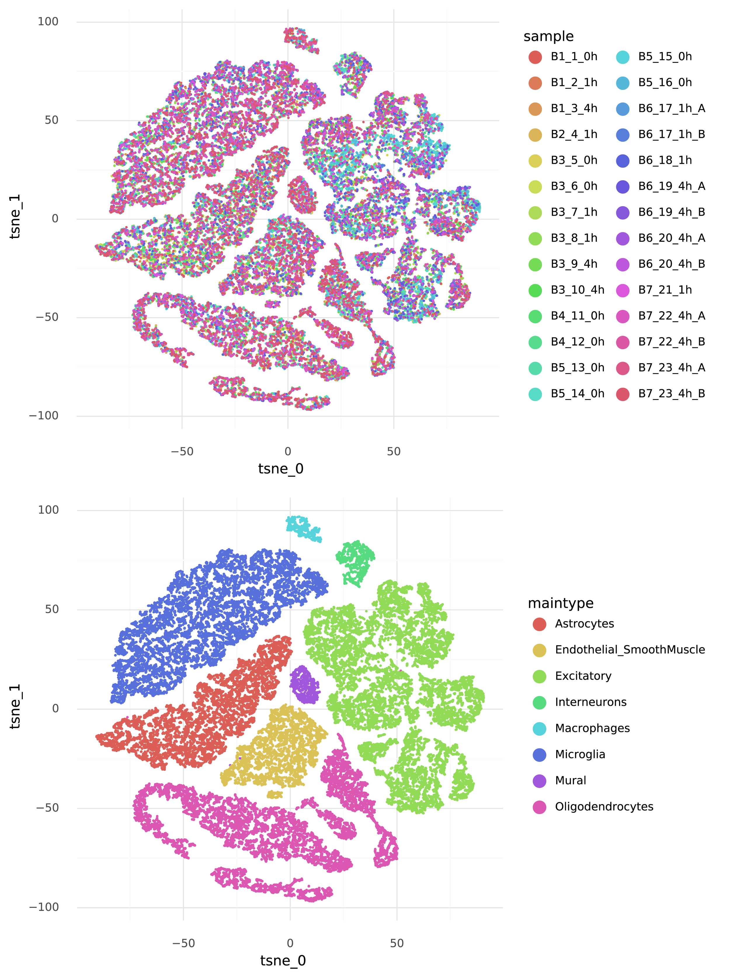
Note how the cells group by cell type, but not by experimental sample.

\( W = f(Z, c) \in \mathbb{R}^{128} \)

scVI is a conditional autoencoder. This is what enables it to find a representation with the variation between batches accounted for. When generating data the first step is to introduce the batch-to-batch variation. This is done by taking a representation \( z_i \) and the batch \( c_i \) of the \( i \)’th cell, passing these through a neural network \( f() \), and producing an intermediate representation \( w_i \). As above, cells with similar 128-dimensional \( w_i \) representations will produce similar transcriptome observations. Again, we cannot feasibly visualize the 128-dimensional representation of the data, but we can produce a tSNE visualization which allows us to see which cells are close together.

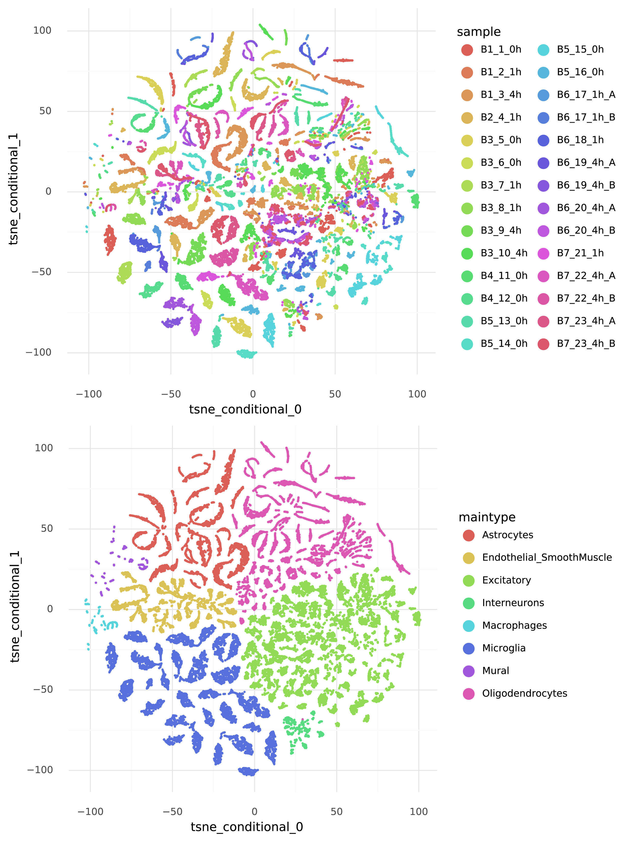
Note that compared to the previous tSNE, here cells from the same biological replicate are lumped together. But this happens within variation due to cell type.

\( X = g(W) \in \mathbb{R}^{25,187} \)

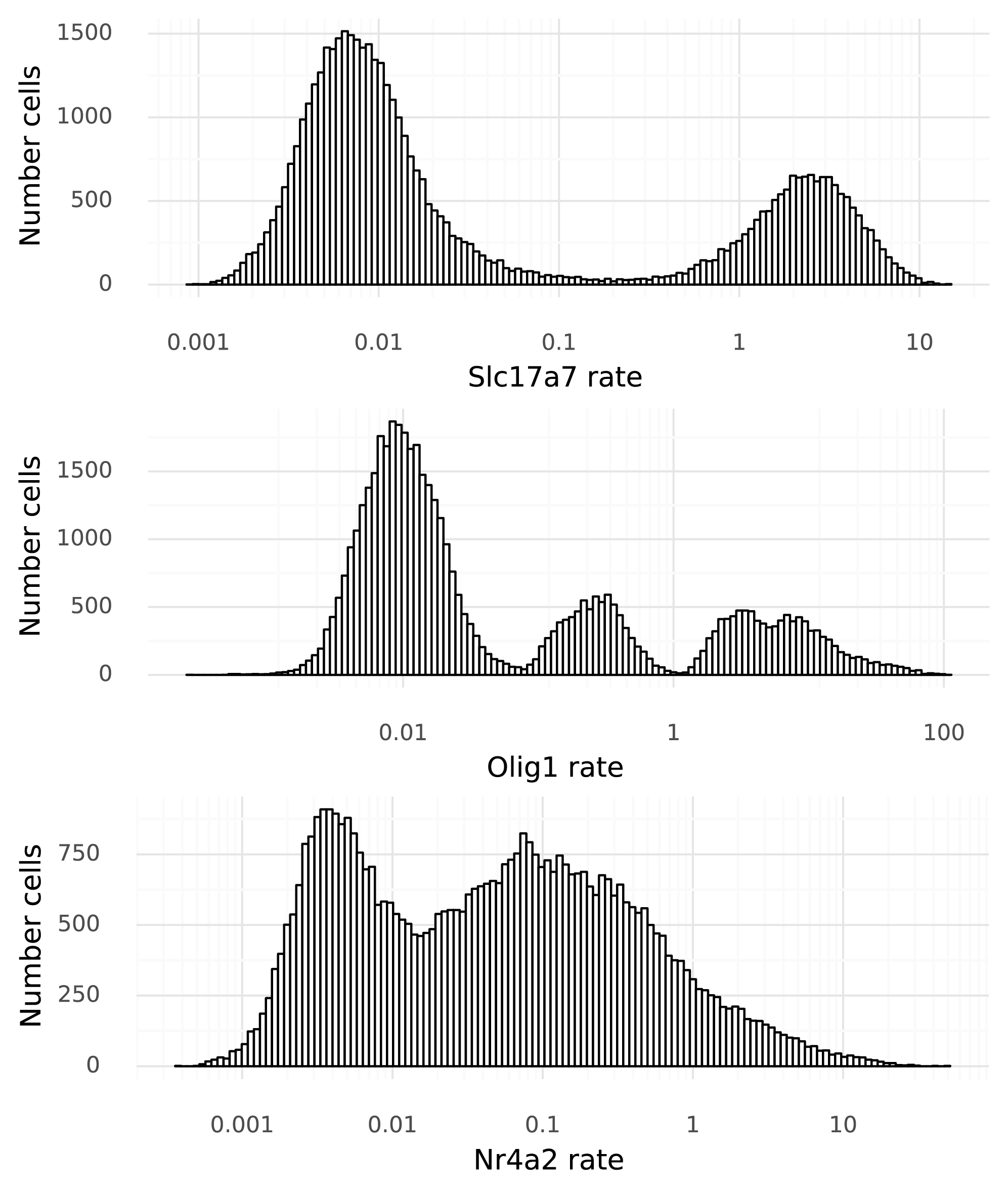
At last, it is time to start to tie gene expression to the cells. To move from the 128-dimensional representation of the cells, a neural network \( g() \) is used to produce one real value per gene in that cell. For this particular dataset each \( x_i \) is 25,187-dimensional. Below figure shows the distribution of these \( x_i \) values for the three example genes across the 48,266 cells in the dataset.

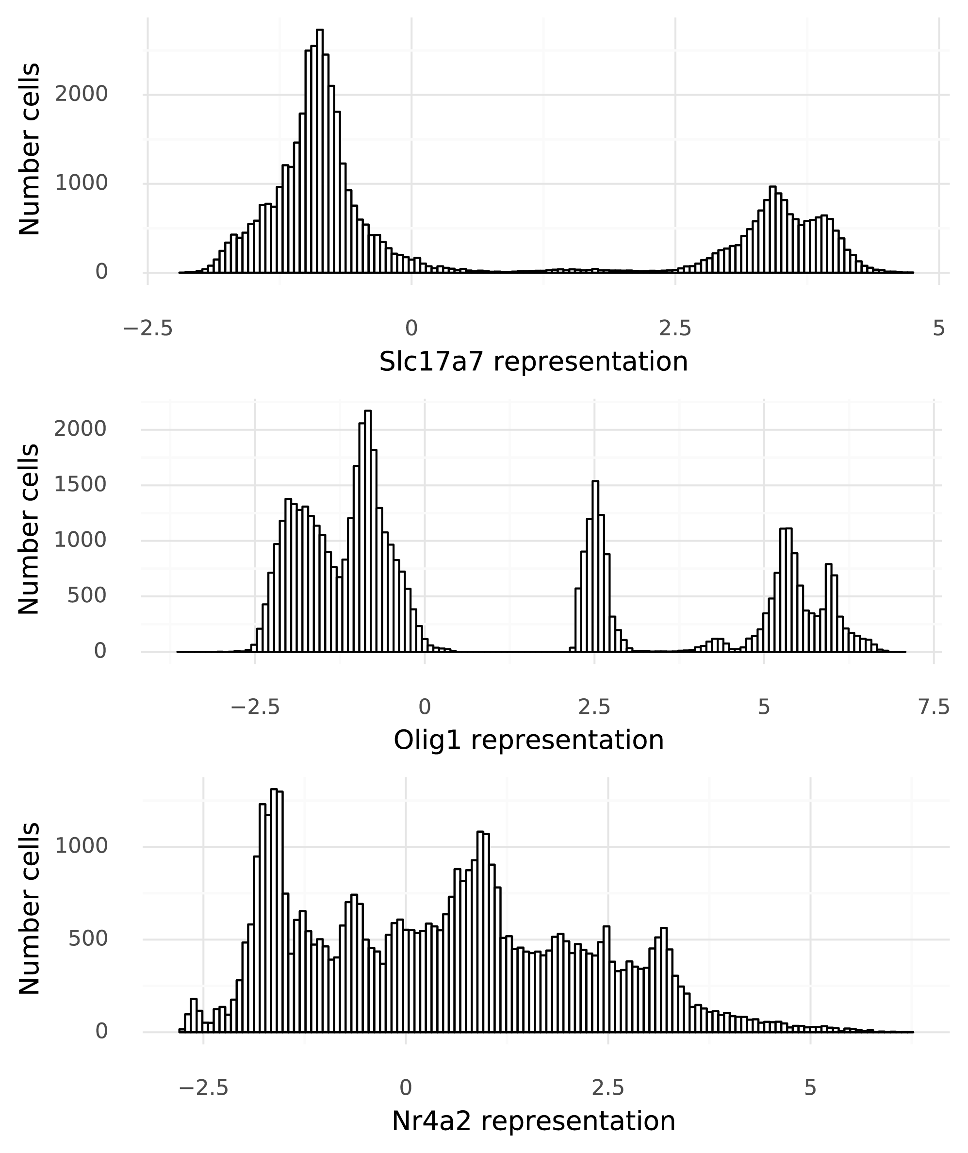
Now variation in gene expression levels can be investigated. This is particularly clear in the bimodal nature of Slc17a7 expression, owing to the mixture of excitatory neurons and other cells. However, these numbers (on the x-axis) that are produced by \( g() \) have no direct ties to the observed data. It is not clear what a value of 3.0 means, for example. This step is here simply because naive neural networks can only map values to unrestricted real numbers. The next step remedies this.

\( \omega = softmax(X) \in \Delta^{25,187} \)

The original data is in UMI counts, and counts are modeled through frequencies and rates. To obtain a frequency from the \( X \)-values, scVI performs a softmax transformation so that the resulting \( \omega_i \) value for each cell sums to 1. The softmax transformation is defined as

\[ \omega_{i, g} = softmax(X_{i, g}) = \frac{\exp(X_{i, g})}{\sum_{k=1}^G \exp(X_{i, k})}. \]

Thus, each \( \omega_i \) lies on the simplex \( \Delta^{25,187} \). Now scVI has generated a value we can interpret.

The frequency \( \omega_{i, g} \) means that every time we would count a molecule in cell \( i \), there is a \( \omega_{i, g} \) chance that the molecule was produced by gene \( g \). These (latent) frequencies are the most useful values produced in scVI, and allows for differential expression analysis as well as representing gene expression on an easily interpretable scale. By convention, the frequencies can be multiplied by 10,000 to arrive at a unit of “expected counts per 10k molecules” for genes. This is similar to the idea behind TPM as a unit in bulk RNA-seq.

\( \Lambda = \omega \cdot \ell \in \mathbb{R}^{25,187} \)

To be able to generate samples similar to the observed data, another technical source of variation needs to be added. Different cells have a different total number of UMI’s. The frequencies above represent how likely we are to observe a molecule from a given gene when sampling a single molecule. The rate \( \Lambda_{i, g} \) represent the expected number of molecules produced by gene \( g \) in cell \( i \) when sampling \( \ell_i \) molecules. This value \( \ell \) is usually referred to as the “library size” or “total UMI counts”. (In scVI \( \ell_i \) is also a random variable, but this is a detail that is not important for the general concept described here.)

In analysis of scRNA-seq data, the total UMI count per cell is easily influenced by technical aspects of data. Unlike frequencies, the scales for a given gene are not directly comparable between cells.

\( Y \sim \text{NB}(\Lambda, \theta) \in \mathbb{N}_0^{25,187} \)

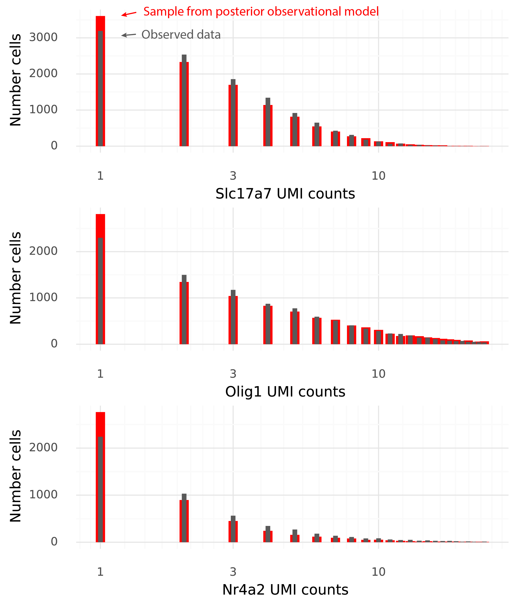
Finally, using the rates \( \Lambda_{i, g} \), the observational negative binomial model can be used to draw samples of UMI counts per cell \( i \) and gene \( g \). (The additional dispersion parameter \( \theta \) can be estimated with a number of different strategies in scVI, and can be considered a detail here).

This is the final step which makes the model generative. At this point, the goal is that a sample from the model with the inferred \( \Lambda \) from the entire dataset should be easily confused with the observed data. The below figure shows histograms for the three example genes of the observed data in grey, and from a sample from the scVI model in red.

An even better strategy to illustrate these properties is to draw multiple samples and see whether the observed data falls within certainty intervals of the sampled data. In the figure below each red line corresponds to a histogram value from a sample from the observational model.

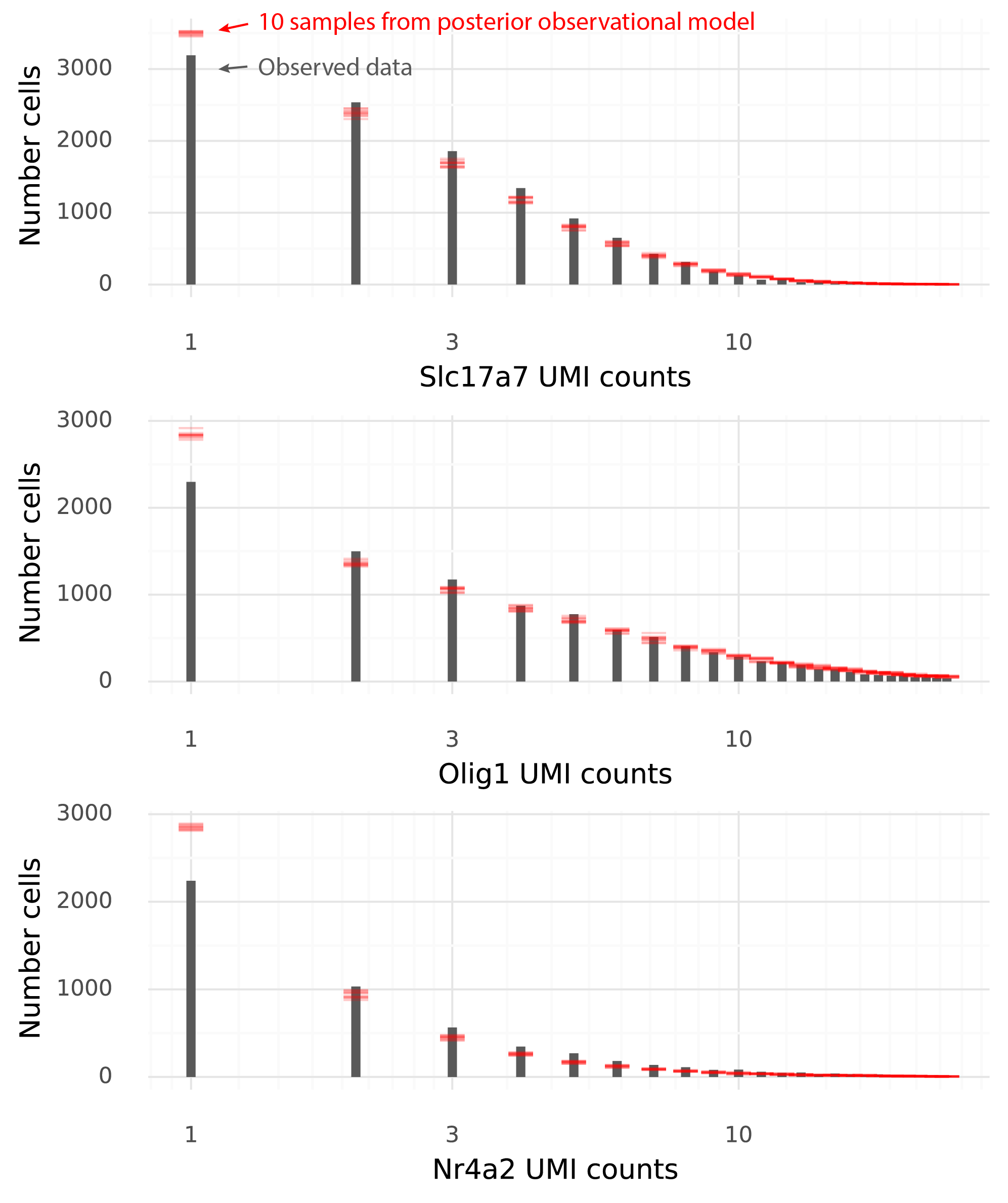
The data and the samples have pretty similar distributions. Some aspects of the observed data are not seen in the samples from the observational model. In particular data sampled from the observational model produce more 1-counts for these three genes than what was observed in the data.

(It should be noted that here samples have only been taken at the last step, from the observational negative binomial model. To perform a posterior predictive check, \( Z \)-values should also be sampled from the approximate posterior of \( Z \).)

The aim of this post has been to show how in scVI the representation \( Z \), which can be used for many cell-similarity analyses is directly tied to gene expression. And the gene expression in turn is directly tied to the sparse UMI counts that are observed through single cell RNA-sequencing. These links are very difficult to make in other analysis methods or 'pipelines' of analysis.

A Juptyer notebook that illustrates how to generate all the quantities described here and all the figures is available on Github