Disappointing variational inference for GLMM's

Generalized linear mixed models (GLMMs) are fantastic tools for analyzing data with complex groupings in measurements. With a GLMM, one can write a model so that population level effects can be investigated and compared, while accounting for variation between groups within the population. As the number of population effects one wants to compare increases, and the size of the input data increases, the models take more time to fit.

In Boland et al 2020 the authors compared mRNA expression in cells from blood and rectum from healthy people and patients with ulcerative colitis (UC). They found that T cells (specifically regulatory T cells) from rectum of UC patients had enriched expression of ZEB2. Estimating the expression levels of ZEB2 in the different conditions in this data is a good example of how GLMM's can be used.

All the 68,627 cells in the Boland et al 2020 data can be divided into 20 cell groups of interest from the triplets (5 cell types, 2 tissues, 2 disease states). The cells were collected from 7 UC patients and 9 healthy people. Naturally, disease state is confounded with patient identity: with a regular generalized linear model it is not possible to account for patient-to-patient variation while estimating the disease state specific expression. However, with a GLMM, the patient-specific effect on the expression level can be considered a random effect while the disease state-specific expression level is a population effect. The GLMM for ZEB2 counts \( Y \) can be written as:

$$ \begin{align} \mu_\text{patient} &\sim \text{N}(0, \sigma_\text{patients}), \\ \lambda &= \exp(\mu_\text{cell group} + \mu_\text{patient} ) \cdot s, \\ Y &\sim \text{Poisson}(\lambda), \end{align} $$

where ( s ) is the UMI count depth per cell. This model can be fitted with the lme4 R package using the formula ZEB2 ~ 0 + cell_group + offset(log(total_count)) + (1 | patient_assignment). In the context of single cell RNA-seq data, this problem is relatively simple. There are only 20 fixed (population) effects, and 18 random effects, with ~70,000 observations. But it still takes over 15 minutes to fit this model of ZEB2 expression using lme4.

A popular method to scale model fitting is variational inference. Variational inference is a Bayesian method, so priors need to be specified:

$$ \begin{align} \sigma_\text{patients} &\sim \text{HalfNormal}(0, 1), \\ \mu_\text{cell group} &\sim \text{N}(0, 1) \end{align} $$

Tensorflow-probability (TFP) has a tutorial on how to fit GLMMs with variational inference on their website. The example code provided can be modified to implement the model defined above for the Boland et al 2020 data.

Unlike the parameter fitting algorithm in lme4, variational inference in TFP involves stochastic steps. To compare the results from lme4 with the results from the TFP model it is necessary to fit the TFP model several times to see how much the results vary between runs. Here, the TFP GLMM implementation was fitted on the Boland et al 2020 data 10 times.

The main goal is to obtain accurate estimates with uncertainty for the population level effects (the cell group means). Secondarily, it is good if the fits for the means of the random effects are accurately estimated.

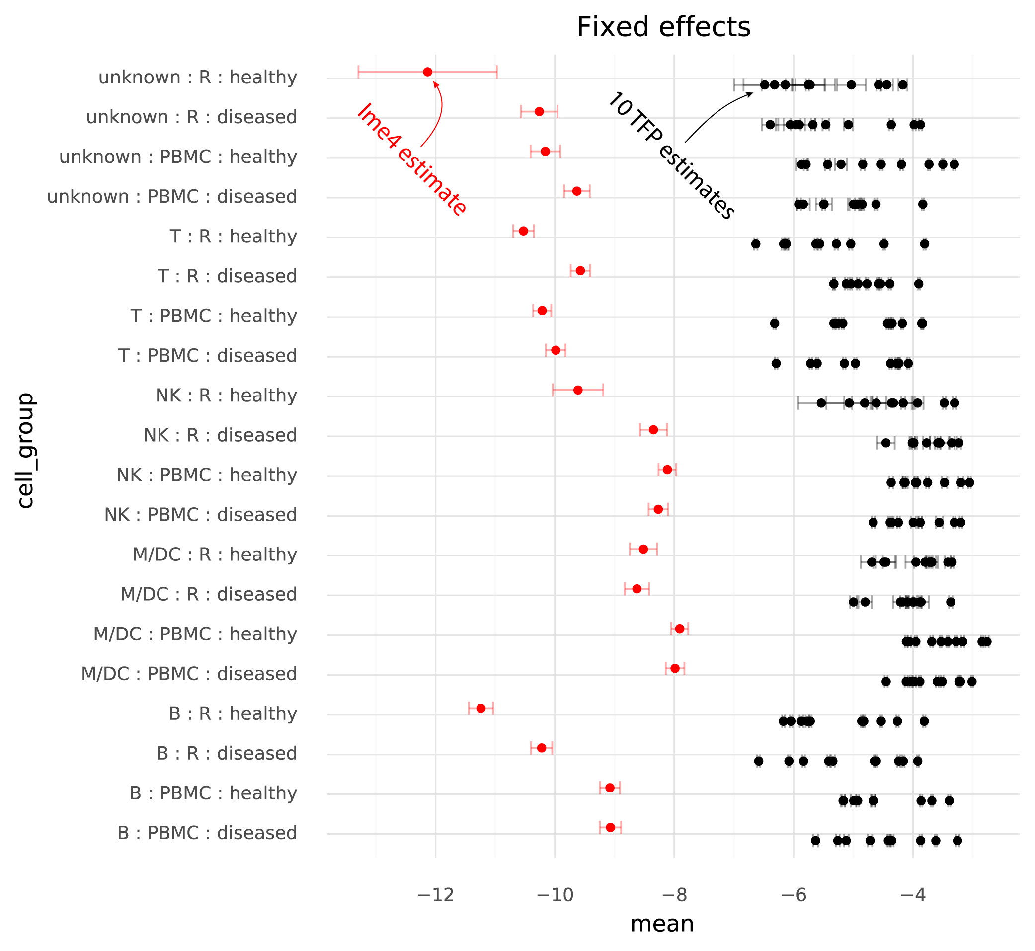
Below are the estimated cell group means from lme4, and the 10 runs of TFP.

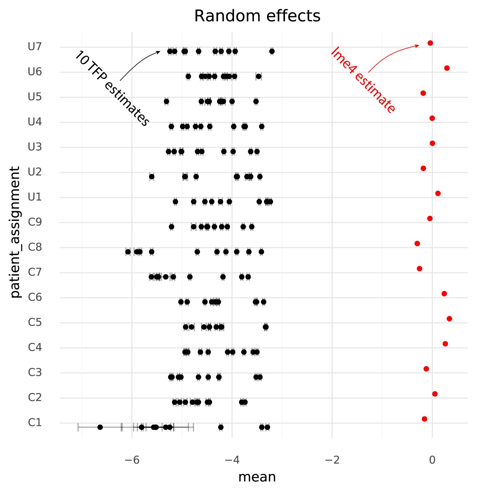
One immediately clear issue here is that there is a bias in the TFP estimates compared to the lme4 estimates. Looking at the random effects reveals the reason for this.

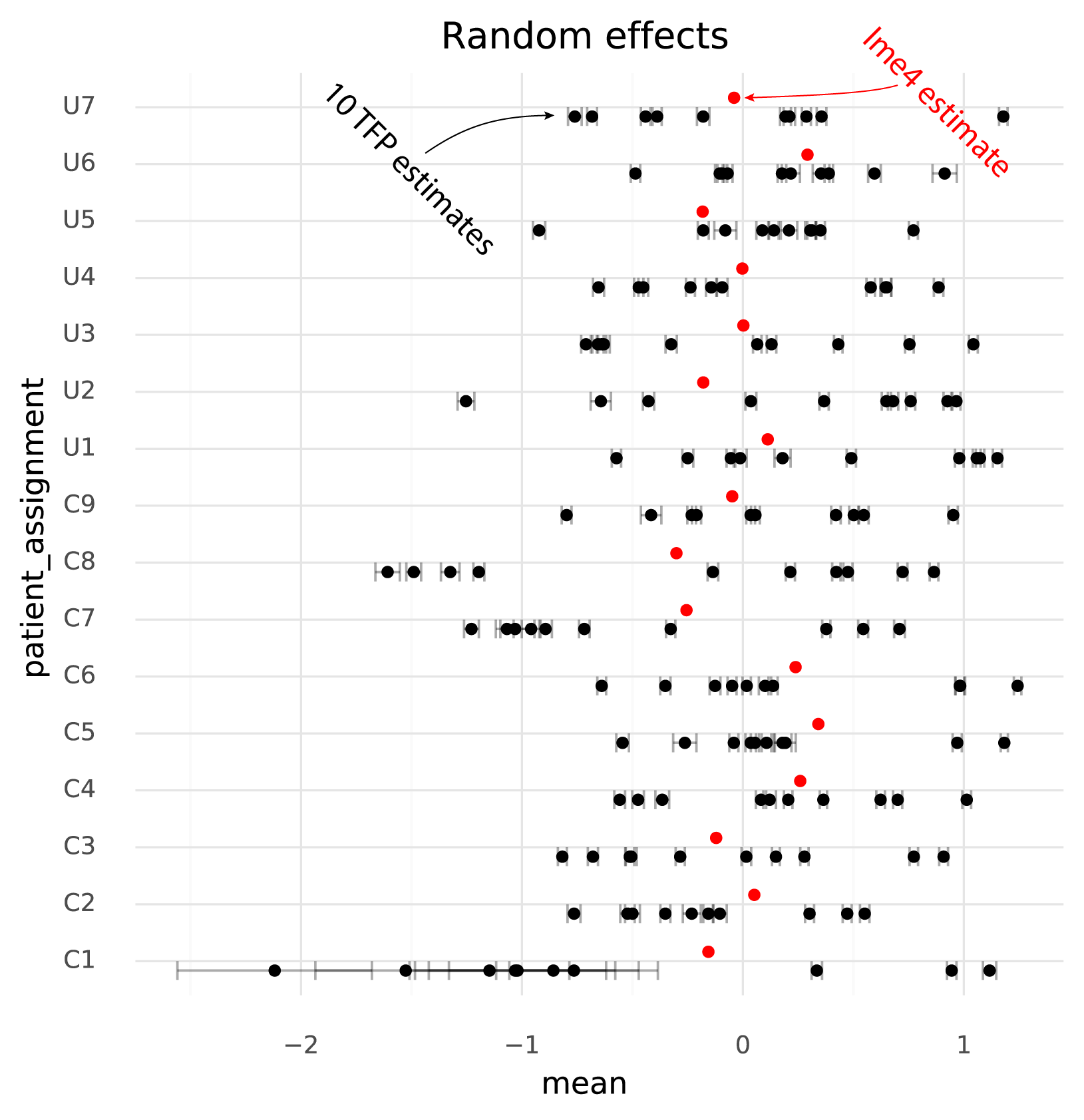
Even though the model specified \( \mu_\text{patient} \sim \text{N}(0, \sigma_\text{patients}) \) the TFP fits find a non-zero mean for the random effects. This might be an effect of the \( \text{N}(0, 1) \) prior on the fixed effects, causing the estimates both for the fixed and random effects to be shifted to satisfy both priors.

The units of the estimated fixed effects from TFP can be made comparable with the units from lme4 by shifting by the mean of the estimated random effects from TFP, since in the lme4 results the random effects have mean 0.

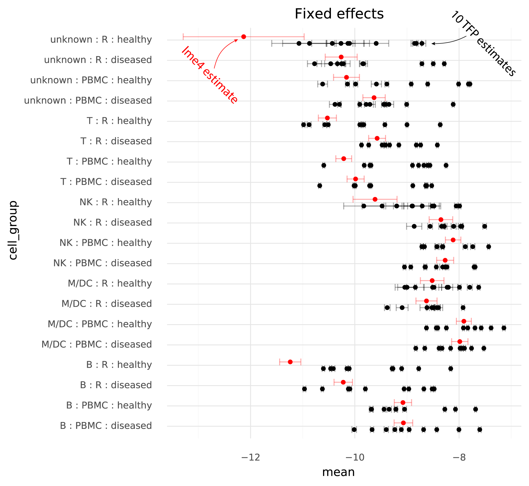
The following plot shows TFP fixed effect estimates on the transformed scale where the means of the random effects are 0:

On this common scale (where the unit is “log probability of observing a ZEB2 molecule when sampling a molecule from the given cell group population”), there are two particularly clear issues. First, the whiskers on the plots show the +/- 2 * standard deviation of the estimates. The standard deviation of the lme4 estimates are obtained from the curvature of the likelihood function. The standard deviations from TFP are parameters which are fitted by the variational inference method. TFP standard deviations are much smaller than the standard deviations from lme4, reflecting a known property of variational inference.

Secondly, and more problematically, there is a huge amount of variation between runs of variational inference with TFP. This variation is much larger than the uncertainty in the lme4 estimate, and often changes the relative difference between two cell groups. That is, if one wants to calculate a contrast between two populations to perform a differential expression analysis, different runs of variational inference will result in negative or positive fold changes randomly.

This is disappointing, because these limitations are not discussed in the TFP tutorial on GLMM's. Instead, the TFP tutorial gives the impression that it 'just works', even without tuning the model.

Jupyter notebooks, R code, as well as a CSV file with ZEB2 expression data, are available at GitHub.