Tutorial - Label transfer with scVI and scHPL
One of the most time-consuming and challenging steps in single-cell RNA-seq analysis is the assignment of cell types based on clustering marker genes. There are numerous variations on settings, all equally valid but slightly different, and never align perfectly with expected biology. This challenge is compounded by the ambiguous literature regarding which marker genes should appear where.
To leverage the hard work that has already been done, strategies for label transfer have been developed. In this scenario, unlabeled data is labeled based on its similarity to already labeled cells.
The scHPL package (Michielsen, Reinders, and Mahfouz 2021; Michielsen et al. 2022) is an excellent tool for this task. It uses k-nearest neighbor classifiers and incorporates a powerful feature that takes into account a tree structure of cell type labels. This approach not only enables the use of known labels at a lower resolution than some other labels but also prevents overly confident label transfers for highly resolved sub-labels that may not be realistic.
Although this tool is generally straightforward to use, it requires some initial setup in the form of upstream tasks. Some helper code can also make it more approachable.
ImYoo, a biotech startup (www.imyoo.health), has provided a pre-labeled scRNA-seq dataset. This dataset, composed of capillary blood samples self-collected by three participants. Included are their custom labels, specifically incorporated for creating a comprehensive tutorial on label transfer using tools such as scVI and scHPL. Those interested in exploring rich single-cell gene expression datasets, particularly those related to the human immune system, or seeking more information on decentralized blood sampling, are encouraged to contact ImYoo through their website.
To start, you’ll need to import a number of packages that will be used throughout the tutorial.
import anndata
import numpy as np
import pandas as pd
import plotnine as p
import matplotlib.pyplot as plt
import scvi
from scvi.model.utils import mde
import scHPL
import torch

import matplotlib.pyplot as plt
%matplotlib inline
%config InlineBackend.figure_format='retina'

import warnings
warnings.filterwarnings('ignore')
from IPython.display import display
With these packages, you can proceed to read data stored in the h5ad format.
adata = anndata.read_h5ad('imyoo_capillary_blood_samples_76535_pbmcs.h5ad')
adata

AnnData object with n_obs × n_vars = 87213 × 36601
    obs: 'barcode', 'Sample IDs', 'Participant IDs', 'Cell Barcoding Runs', 'cell_type_level_1', 'cell_type_level_2', 'cell_type_level_3', 'cell_type_level_4'
    var: 'name', 'id'
This dataset has 87,000 cells sourced from three independent donors, which have been processed over multiple experimental samples.
adata.obs['Participant IDs'].value_counts()

Participant IDs
3     49170
2     30917
51     7126
Name: count, dtype: int64
In this tutorial, we assume that the cell type labels for participants 2 and 3 are known, and the goal is to transfer these labels to participant 51.
Participant IDs are confounded with Sample IDs. To make cell type labels consistent across participants and experimental samples, you will need to learn an scVI cell representation where variation due to Sample IDs is removed.
scvi.model.SCVI.setup_anndata(
    adata,
    batch_key = 'Sample IDs',
)
Once the AnnData dataset has been set up for scVI, you can proceed to construct an scVI model.
model = scvi.model.SCVI(
    adata,
    n_layers = 2,
    gene_likelihood = 'nb'
)

model.view_anndata_setup()

Anndata setup with scvi-tools version 0.20.3.


Setup via `SCVI.setup_anndata` with arguments:


{
│   'layer': None,
│   'batch_key': 'Sample IDs',
│   'labels_key': None,
│   'size_factor_key': None,
│   'categorical_covariate_keys': None,
│   'continuous_covariate_keys': None
}


        Summary Statistics
┏━━━━━━━━━━━━━━━━━━━━━━━━━━┳━━━━━━━┓
┃     Summary Stat Key     ┃ Value ┃
┡━━━━━━━━━━━━━━━━━━━━━━━━━━╇━━━━━━━┩
│         n_batch          │  32   │
│         n_cells          │ 87213 │
│ n_extra_categorical_covs │   0   │
│ n_extra_continuous_covs  │   0   │
│         n_labels         │   1   │
│          n_vars          │ 36601 │
└──────────────────────────┴───────┘


              Data Registry
┏━━━━━━━━━━━━━━┳━━━━━━━━━━━━━━━━━━━━━━━━━━━┓
┃ Registry Key ┃    scvi-tools Location    ┃
┡━━━━━━━━━━━━━━╇━━━━━━━━━━━━━━━━━━━━━━━━━━━┩
│      X       │          adata.X          │
│    batch     │ adata.obs['_scvi_batch']  │
│    labels    │ adata.obs['_scvi_labels'] │
└──────────────┴───────────────────────────┘


                    batch State Registry
┏━━━━━━━━━━━━━━━━━━━━━━━━━┳━━━━━━━━━━━━┳━━━━━━━━━━━━━━━━━━━━━┓
┃     Source Location     ┃ Categories ┃ scvi-tools Encoding ┃
┡━━━━━━━━━━━━━━━━━━━━━━━━━╇━━━━━━━━━━━━╇━━━━━━━━━━━━━━━━━━━━━┩
│ adata.obs['Sample IDs'] │     20     │          0          │
│                         │     95     │          1          │
│                         │    329     │          2          │
│                         │    424     │          3          │
│                         │    892     │          4          │
│                         │    894     │          5          │
│                         │    909     │          6          │
│                         │    911     │          7          │
│                         │    952     │          8          │
│                         │    953     │          9          │
│                         │    958     │         10          │
│                         │    959     │         11          │
│                         │    970     │         12          │
│                         │    971     │         13          │
│                         │    977     │         14          │
│                         │    978     │         15          │
│                         │    1004    │         16          │
│                         │    1005    │         17          │
│                         │    1071    │         18          │
│                         │    1072    │         19          │
│                         │    1170    │         20          │
│                         │    1171    │         21          │
│                         │    1176    │         22          │
│                         │    1177    │         23          │
│                         │    1382    │         24          │
│                         │    1385    │         25          │
│                         │    1394    │         26          │
│                         │    1395    │         27          │
│                         │    1553    │         28          │
│                         │    1585    │         29          │
│                         │    1593    │         30          │
│                         │    1643    │         31          │
└─────────────────────────┴────────────┴─────────────────────┘


                    labels State Registry
┏━━━━━━━━━━━━━━━━━━━━━━━━━━━┳━━━━━━━━━━━━┳━━━━━━━━━━━━━━━━━━━━━┓
┃      Source Location      ┃ Categories ┃ scvi-tools Encoding ┃
┡━━━━━━━━━━━━━━━━━━━━━━━━━━━╇━━━━━━━━━━━━╇━━━━━━━━━━━━━━━━━━━━━┩
│ adata.obs['_scvi_labels'] │     0      │          0          │
└───────────────────────────┴────────────┴─────────────────────┘
This model is designed to learn a representation for the 87,000 cells, where variation due to the 32 Sample IDs has effectively been eliminated by treating each Sample ID as a separate batch.
With 87,000 cells, running the model for 50 epochs will allow it to process just over four million examples during the fitting process. This should be more than sufficient to reach convergence, a good rule of thumb being to allow a model to process at least one million examples.
model.train(50, check_val_every_n_epoch = 1)

GPU available: True (cuda), used: True
TPU available: False, using: 0 TPU cores
IPU available: False, using: 0 IPUs
HPU available: False, using: 0 HPUs
LOCAL_RANK: 0 - CUDA_VISIBLE_DEVICES: [0]
Epoch 50/50: 100%|█████████████████████████████████████████████████████████████████████████████████████████████████████████████████████████████████| 50/50 [12:45<00:00, 15.51s/it, loss=7.36e+03, v_num=1]
`Trainer.fit` stopped: `max_epochs=50` reached.
Epoch 50/50: 100%|█████████████████████████████████████████████████████████████████████████████████████████████████████████████████████████████████| 50/50 [12:45<00:00, 15.31s/it, loss=7.36e+03, v_num=1]
To ensure the effectiveness of the model fitting, examining the loss curves over the training period is advisable. These curves indicate whether the model is converging as well as highlight if there are issues with overfitting.
history_df = (
    model.history['elbo_train'].astype(float)
    .join(model.history['elbo_validation'].astype(float))
    .reset_index()
    .melt(id_vars = ['epoch'])
)

p.options.figure_size = 6, 3

p_ = (
    p.ggplot(p.aes(x = 'epoch', y = 'value', color = 'variable'), history_df.query('epoch > 0'))
    + p.geom_line()
    + p.geom_point()
    + p.scale_color_manual({'elbo_train': 'black', 'elbo_validation': 'red'})
    + p.theme_minimal()
)

p_.save('fig1.png', dpi = 300)

print(p_)The decrease in loss between epochs 40 and 50 is extremely small, with the validation loss showing stability. With this level of performance, the model is now ready to estimate representation vectors for all the 87,000 cells.
adata.obsm['X_scvi'] = model.get_latent_representation(adata)To aid in visualizing the representations, the PyMDE package can be utilized to generate a 2D representation of the neighborhood graph of the scVI representation vectors. This package is conveniently available as a utility within scvi-tools.
adata.obsm['X_mde'] = scvi.model.utils.mde(adata.obsm['X_scvi'])

for i, y in enumerate(adata.obsm['X_mde'].T):
    adata.obs[f'mde_{i + 1}'] = y
The labels in the dataset are organized in four columns, each representing different levels. Some cells may only be labeled in the second column, without labels in the third or fourth columns. Conversely, some cells might have labels in all four columns. Absence of labels is indicated by NaNs.
(
    adata
    .obs
    .groupby(
        ['cell_type_level_1', 'cell_type_level_2', 'cell_type_level_3', 'cell_type_level_4'],
        observed = True,
        dropna = False
    )
    .size()
    .rename('#')
    .reset_index()
)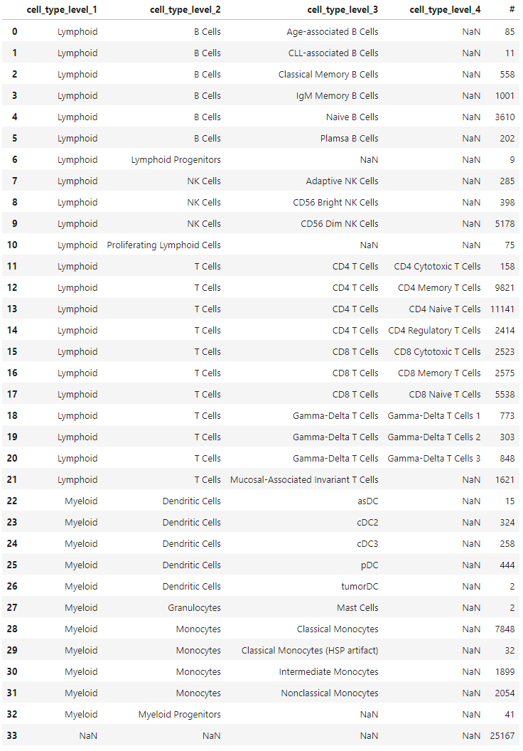
In order to make this label structure compatible with scHPL, there needs to be a single column of labels for each cell, along with a separate tree structure that indicates how these labels relate to each other. Moreover, cells without specific labels must be labeled as ‘root’ in order for scHPL to function properly. This label indicates that the cell can originate from any branch of the tree.
for i in range(1, 4 + 1):
    adata.obs[f'cell_type_level_{i}'] = adata.obs[f'cell_type_level_{i}'].pipe(np.array)

# Propagate upper level labels

adata.obs.loc[adata.obs.query('cell_type_level_1.isna()').index, 'cell_type_level_1'] = 'root'
If a cell has a label in a column representing a higher level, but lacks a label at the current level, the label from the higher level must be propagated to the next level.
for i in range(2, 4 + 1):
    idx_ = adata.obs.query(f'cell_type_level_{i}.isna()').index
    adata.obs.loc[idx_, f'cell_type_level_{i}'] = adata.obs.loc[idx_][f'cell_type_level_{i - 1}'].values

(
    adata
    .obs
    .groupby(
        ['cell_type_level_1', 'cell_type_level_2', 'cell_type_level_3', 'cell_type_level_4'],
        observed = True,
        dropna = False
    )
    .size()
    .rename('#')
    .reset_index()
)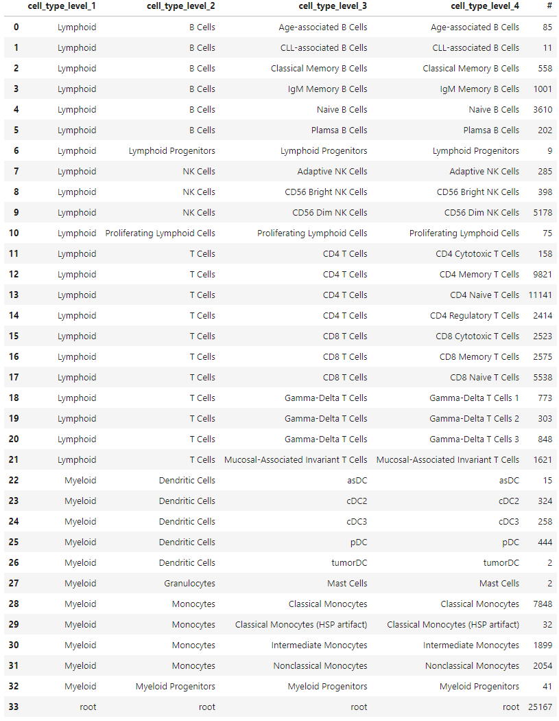
The reformatted label structure encapsulates all necessary information about the cell type labels encoded in the fourth column, eliminating any NaNs.
The tree structure, which can be visually understood from the grouped summary table, must be represented by a precise tree data structure. This can be achieved by encoding the structure as a nested set of dictionaries.
# Empty dicts indicates leaves.
tree = {
    'root': {
        'Lymphoid': {
            'T Cells': {
                'Mucosal-Associated Invariant T Cells': {},
                'Gamma-Delta T Cells': {
                            'Gamma-Delta T Cells 1': {},
                            'Gamma-Delta T Cells 2': {},
                            'Gamma-Delta T Cells 3': {},
                },
                'CD8 T Cells': {
                            'CD8 Memory T Cells': {},
                            'CD8 Cytotoxic T Cells': {},
                            'CD8 Naive T Cells': {},
                },
                'CD4 T Cells': {
                            'CD4 Naive T Cells': {},
                            'CD4 Memory T Cells': {},
                            'CD4 Regulatory T Cells': {},
                            'CD4 Naive T Cells': {},
                            'CD4 Regulatory T Cells': {},
                            'CD4 Cytotoxic T Cells': {}
                }
            },

            'NK Cells': {
                'CD56 Dim NK Cells': {},
                'Adaptive NK Cells': {},
                'CD56 Bright NK Cells': {}
            },
            'B Cells': {
                'Naive B Cells': {},
                'IgM Memory B Cells': {},
                'Plamsa B Cells': {},
                'Age-associated B Cells': {},
                'Classical Memory B Cells': {},
                'CLL-associated B Cells': {},
            },
            'Lymphoid Progenitors': {}
        },
        'Myeloid': {
            'Monocytes': {
                'Classical Monocytes': {},
                'Intermediate Monocytes': {},
                'Classical Monocytes HSP artifact': {},
                'Nonclassical Monocytes': {}
            },
            'Dendritic Cells': {
                'asDC': {},
                'pDC': {},
                'cDC3': {},
                'tumorDC': {}
            },

            'Granulocytes': {
                'Mast Cells': {}
            },
            'Myeloid Progenitors': {}
        }
    }
}
scHPL utilizes trees defined in the Newick format to construct a tree structure of classifiers. The nested dictionary structure can be conveniently converted into a Newick string using a small helper function.
# This lets you define trees as a dict of dicts. It converts it to a Newick string that you can give to scHPL

def dict2newick(tree, name):

    if len(tree[name]) == 0:
        return f'{name}'

    else:
        child_strings = [dict2newick(tree[name], child) for child in tree[name]]
        return f'({", ".join(child_strings)}){name}'

tree1 = scHPL.utils.create_tree(dict2newick(tree, 'root'))
Once the scHPL tree has been created, a graphical representation can be plotted to verify the accuracy of the structure.
scHPL.utils.print_tree(tree1)The tree structure, now delineating the relationship between the different cell type labels, facilitates the training of a tree of k-nearest neighbor classifiers using these labels in scHPL. In the continuous scVI embedding space, cells with similar vectors will produce statistically compatible UMI counts. Cell types within this space will manifest as dense regions of embedded cells, but without any expectation that these regions are linearly separable, which makes k-nearest neighbor classifiers a compelling choice for label transfer. k-nearest neighbor classifiers are also highly resistant to class imbalance, particularly for small k values with large volumes of training data. Cell types are often significantly imbalanced due to biology; for example, in this dataset 70% of the cells are T cells.
Before starting the training process, labels from participant 51, which are assumed to be unknown in this tutorial, need to be renamed to ‘Unknown’ (or some other arbitrary name).
adata.obs['tree_label'] = adata.obs['cell_type_level_4']

# We are ignoring known labels for participant 51, so here we rename these

adata.obs.loc[adata.obs.query('`Participant IDs` == 51').index, 'tree_label'] = 'Unknown'

adata.obs['participant_ids'] = adata.obs['Participant IDs']
Equipped with these labels, we can visualize the cells’ representations along with their given labels using scatter plots.
p.options.figure_size = 12, 15

tmp_ = adata.obs.sample(20_000)

p_ = (
    p.ggplot(p.aes(x = 'mde_1', y = 'mde_2', color = 'tree_label'), tmp_)
    + p.geom_point(shape = '.', size = 0.1, color = 'lightgrey', data = tmp_.drop(['participant_ids'], axis = 1))
    + p.geom_point(shape = '.', size = 0.2)
    + p.theme_minimal()
    + p.guides(color = p.guide_legend(override_aes = {'size': 10}))
    + p.facet_grid('participant_ids ~ .', labeller = 'label_both')
)

p_.save('fig3.png', dpi = 300)

print(p_)When initiating the training process for the tree, the data from participant 51 is deliberately excluded.
adata_train = adata[adata.obs.query('participant_ids != 51').index].copy()Finally, the cell representations from scVI, the known labels, and the tree structure of the labels, are all fed into the training function in scHPL. This process generates a trained classifier tree.
trained_tree = scHPL.train_tree(
    adata_train.obsm['X_scvi'],
    adata_train.obs['tree_label'],
    tree1,
    dimred = False,  # These two options for compatibility with scVI
    useRE = False
)
Once trained, the classifier tree can be applied to all cells to generate their predicted labels.
adata.obs['predicted_label'] = scHPL.predict_labels(adata.obsm['X_scvi'], trained_tree)Comparing the results of the label transfer with the given labels allows for an assessment of their consistency with their continuous scVI representation vectors. A confusion matrix is an ideal tool for this, as it displays the distribution of predicted labels for each given label.
Since scHPL utilizes the hierarchical structure of the labels, and can ‘stop’ at higher levels of labels if lower levels are ambiguous, it is beneficial to order the confusion matrix in a manner that preserves this hierarchical structure. Such ordering can be achieved through a recursive depth-first traversal of the label tree.
def get_depth_first_order(tree):

    label_order = []
    depth = 0 - 1

    def depth_first_order(node, label_order, depth):
        depth += 1
        label_order += [{'name': node.name[0], 'depth': depth}]

        for child in node.descendants:
            depth_first_order(child, label_order, depth)

        depth -= 1

    depth_first_order(tree[0], label_order, depth)

    return pd.DataFrame(label_order).reset_index().rename(columns = {'index': 'order'})

label_order = get_depth_first_order(tree1)

scHPL.evaluate.heatmap(
    adata.obs['tree_label'],
    adata.obs['predicted_label'],
    order_rows = label_order['name'].to_list() + ['Unknown'],
    order_cols = label_order['name'].to_list() + ['Rejection (dist)'],
    shape = (12, 11)
)

for i in label_order.query('depth == 1')['order'].values:
    plt.axhline(i, color = 'black', lw = 1)
    plt.axvline(i, color = 'black', lw = 1)

for i in label_order.query('depth == 2')['order'].values:
    plt.axhline(i, color = 'grey', lw = 0.5)
    plt.axvline(i, color = 'grey', lw = 0.5)

for i in label_order.query('depth == 3')['order'].values:
    plt.axhline(i, color = 'grey', lw = 0.2, ls = (0, (5, 10)))
    plt.axvline(i, color = 'grey', lw = 0.2, ls = (0, (5, 10)))

plt.tight_layout()

plt.savefig('fig5.png', dpi = 300)The majority of the cells are predicted as the lower level label given to the classifier. Cells where the prediction ‘stopped’ at a higher level would be visible below the diagonal, adjacent to the separating lines in the confusion matrix plot. Cells with the given label ‘root’ are distributed among the possible labels in the ‘predicted labels’ axis; it is impossible to determine the accuracy of these predictions as there is no ground truth. Some cells receive the predicted label ‘Rejection (dist)’, indicating that these cells are distant from others to infer their potential label.
Cells bearing the ‘Unknown’ label are also distributed among the possible predicted labels, in line with the objective of this tutorial.
The two-dimensional visualization process can be reiterated with the transferred labels. This time, the cells from participant 51 will also have cell type labels.
p.options.figure_size = 12, 15

tmp_ = adata.obs.sample(20_000)

p_ = (
    p.ggplot(p.aes(x = 'mde_1', y = 'mde_2', color = 'predicted_label'), tmp_)
    + p.geom_point(shape = '.', size = 0.1, color = 'lightgrey', data = tmp_.drop(['participant_ids'], axis = 1))
    + p.geom_point(shape = '.', size = 0.2)
    + p.theme_minimal()
    + p.guides(color = p.guide_legend(override_aes = {'size': 10}))
    + p.facet_grid('participant_ids ~ .', labeller = 'label_both')
)

p_.save('fig4.png', dpi = 300)

print(p_)With this, the task is completed! The transferred labels can be utilized for downstream analysis. For instance, you could compare the proportions of the cell types in participant 51 with the other participants. Alternatively, a differential expression analysis between participant 51 and the other participants could be performed to identify any genes that are uniquely expressed in the samples from the donor, for each cell type.
As a bonus, in this specific case, there were already existing labels for the cells from participant 51. As such, the confusion matrix plot from earlier can be replicated, this time comparing the originally given labels with the transferred labels for this subset of data that wasn’t utilized during the tree training phase.
scHPL.evaluate.heatmap(
    adata.obs.query('participant_ids == 51')['cell_type_level_4'],
    adata.obs.query('participant_ids == 51')['predicted_label'],
    order_rows = label_order['name'].to_list(),
    order_cols = label_order['name'].to_list() + ['Rejection (dist)'],
    title = 'Participant IDs == 51 (held out)',
    shape = (12, 11)
);


for i in label_order.query('depth == 1')['order'].values:
    plt.axhline(i, color = 'black', lw = 1)
    plt.axvline(i, color = 'black', lw = 1)

for i in label_order.query('depth == 2')['order'].values:
    plt.axhline(i, color = 'grey', lw = 0.5)
    plt.axvline(i, color = 'grey', lw = 0.5)

for i in label_order.query('depth == 3')['order'].values:
    plt.axhline(i, color = 'grey', lw = 0.2, ls = (0, (5, 10)))
    plt.axvline(i, color = 'grey', lw = 0.2, ls = (0, (5, 10)))

plt.tight_layout()

plt.savefig('fig6.png', dpi = 300)The transferred labels largely align with the original labels; cells typically reside within their own hierarchical ‘box’, although the resolution is not as consistent as with the data used for training. One notable deviation is the group of NK cells, many of which received labels from T cells. Some gamma-delta T cells are assigned as other T cells. None of the cells annotated as cytotoxic T cells are recognized, and some age-associated B cells cannot be predicted with higher precision than the overarching B cells label.
Although this workflow is somewhat extensive, it offers significant reliability. While the prediction step from scHPL can be time-consuming (it took about 10 minutes for these 87,000 cells), the accuracy and clarity of the outcome makes it a worthwhile effort. The usage of k-nearest neighbor classifiers adds robustness against class imbalance, a common challenge when dealing with cell types in biological samples. Parametric classifiers may be more efficient, but they struggle with class imbalance. By examining the predictions within the hierarchies, users can identify potentially unrealistic subclass definitions. If there is significant mixing between predicted cell types, it suggests that the original labels do not align well with the low-dimensional representation of the cells.
A Jupyter notebook for running the entire workflow is available on Github: https://github.com/vals/Blog/tree/master/230608-scHPL-tutorial
The dataset used for this tutorial is available on Zenodo: https://dx.doi.org/10.5281/zenodo.8020792
Thanks to Eduardo Beltrame for useful feedback on this tutorial, and to ImYoo for providing the dataset.
Michielsen, Lieke, Mohammad Lotfollahi, Daniel Strobl, Lisa Sikkema, Marcel Reinders, Fabian J. Theis, and Ahmed Mahfouz. 2022. “Single-Cell Reference Mapping to Construct and Extend Cell Type Hierarchies.” bioRxiv. https://doi.org/10.1101/2022.07.07.499109.
Michielsen, Lieke, Marcel J. T. Reinders, and Ahmed Mahfouz. 2021. “Hierarchical Progressive Learning of Cell Identities in Single-Cell Data.” Nature Communications 12 (1): 2799. https://doi.org/10.1038/s41467-021-23196-8.