Cells in the center of scVI latent space — What do you mean "heterogeneity"?

When modeling scRNA-seq data with scVI, it is common to notice that some cells of mixed cell types appear in the center of the representation space. Often these are lower quality cells, or in cases where snRNA-seq data is mixed with scRNA-seq data, the snRNA-seq data tend to appear closer towards the middle. This leads to difficulties when assigning cell type labels to these cells, or using label transfer workflows. Why does this happen?

With scVI, gene expression levels in cells are modeled by latent variables, representing their state in a way that is compatible with the observed molecule counts of the transcriptomes. A substantially simplified version of the model can be defined by

$$ \begin{align*} Z &\sim \text{N}(\mathbf{0}, \mathbf{1}), \\ \omega &= f(Z), \\ Y &\sim \text{Poisson}(\omega \cdot \ell). \end{align*} $$

Here $ Z $ is the latent representation of the cells, $ \omega $ are observation probabilities for the genes in the cells, and $ \ell $ are the total observed UMI count depths for the cells. This turns the $ \omega \cdot \ell $ term into rate parameters for the Poisson distribution which is used to generate the UMI counts $ Y $. The goal of scVI is to infer the posterior distribution of $ Z $ given the observed counts $ Y $: $ P(Z \ | \ Y) $.

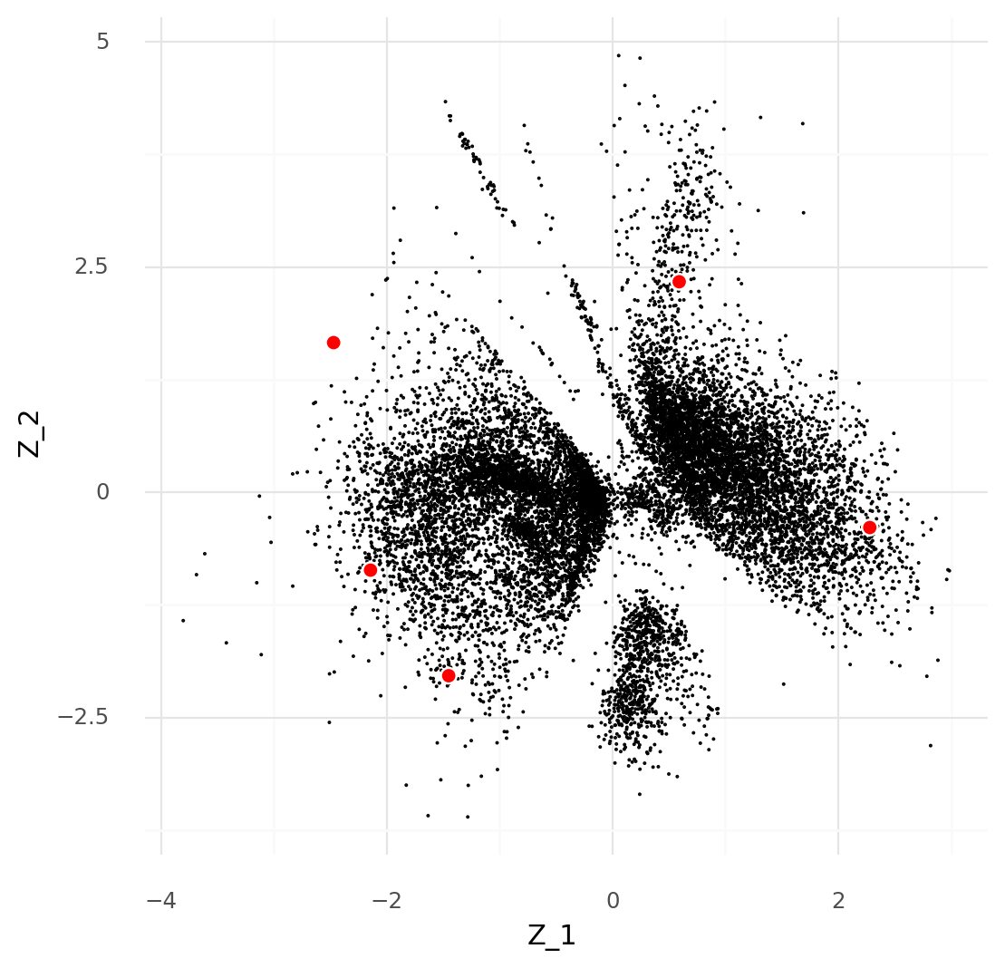
For an illustration, a simple dataset consisting of one sample from (Ren et al. 2021) can be used as in a previous post. This example has 14,545 cells limited to 141 genes known to be markers of various blood cells. Here the scVI model is fitted with a 2-dimensional representation for the sake of a simple visualization.

After fitting the model we get the following plot of the latent representations for the cells:

To investigate the effect of counting fewer mRNA molecules than were actually counted, binomial thinning can be used. The observed counts are used to estimate probabilities of all observations:

$$ P_{c, g} = \frac{Y_{c, g}}{\sum_{g} Y_{c, g}}. $$

These are passed to a binomial distribution where the number of trials are set to the a number $ n $, lower than the observed number, from which new counts are sampled:

$$ \hat{Y}^n \sim \text{B}(n, P). $$

Picking a few cells, these can be binomially thinned to different depths while keeping track of which cells they originated from. These new thinned cells $ \hat{Y}^n $ can be used to infer $ P( \hat{Z}^n \ | \ \hat{Y}^n ) $.

In the plot below five cells were selected for thinning and then used to obtain latent representations $ Z $. The thinned versions of the cells are connected by red lines depending on which their original cell was. These thinned cells are colored by their UMI count depth after thinning.

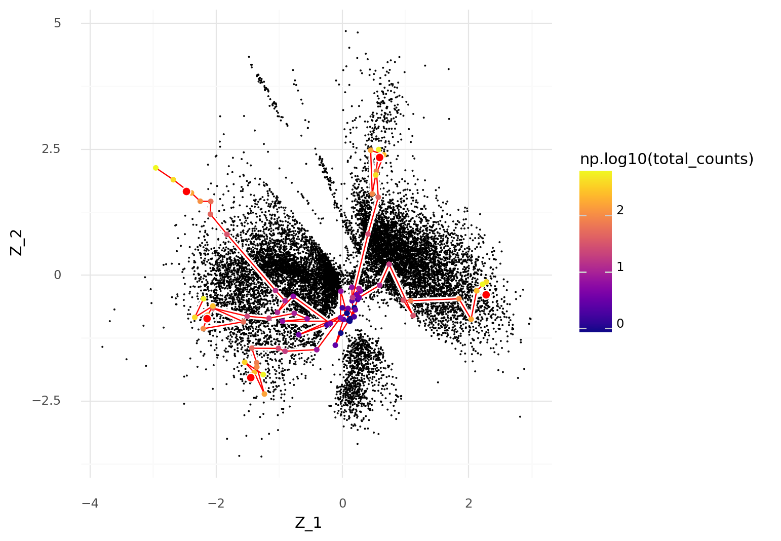
The plot illustrates that as the UMI count depth decreases, the more likely a cell is to be represented by central coordinates, close to the origin, in the scVI latent space.

This effect can be explained by investigating the loss function used for the scVI model. The posterior $ P(Z \ | \ Y) $ is approximated by a parameterized distribution $ Q(Z) $ specifically where $ Q(z_{c, d}) = \text{N}(\mu_{c, d}, \sigma_{c, d}) $ and

$$ \texttt{loss} = \sum_{c, g, d} \left( -\log P(Y | Z) + \text{KL}(Q(Z) || P(Z)) \right). $$

In inference, the loss is minimized. In this particular version with a Poisson likelihood,

$$ \begin{align*} \texttt{log_prob}_c &=\sum_g \log \text{Poisson}(\mathbf{y}_g \ | \ \omega_{c, g} \cdot \ell_c) \\ &= \sum_g \left( \mathbf{y}_g \cdot \log( \omega_{c, g} \cdot \ell_c) - \omega_{c, g} \cdot \ell_c - \log \Gamma (\mathbf{y}_g + 1) \right). \end{align*} $$

It is worth pointing out that $ \ell_c = \sum_g y_{c, g} $ in most situations, so $ \max{\mathbf{y}_g} \leq \ell_c $ The consequence of this is that the $ \texttt{log_prob}_c $ term is limited by the total UMI count depth $ \ell_c $.

The KL term quantifies how far the approximation of the posterior $ Q(Z) $ is from the prior $ P(Z) $. Since the prior consists of unit Gaussian distributions, the KL term is

$$ \begin{align*} \texttt{kl}_c &= \sum_d \text{KL}(Q(\mathbf{z}_d) \ || \ P(\mathbf{z}_d)) \\ &= \sum_d \text{KL}(\text{N}(\mathbf{\mu}_{c, d}, \mathbf{\sigma}_{c, d}) \ || \ \text{N}(0, 1)) = \sum_d \left( -\log \sigma_{c, d} + \frac{{\sigma_{c, d}}^2 + {\mu_{c, d}}^2}{2} - \frac{1}{2} \right). \end{align*} $$

When inferring the approximate posterior $ Q(\mathbf{z}_c) $, the magnitude of $ \texttt{log_prob}_c $ term need to beat the magnitude of the $ \texttt{kl}_c $ term to escape the isotropic unit Gaussian prior $ \text{N}(\mathbf{0}, \mathbf{1}) $.

This can be illustrated by repeating the plot above, but coloring the thinned cells by the $ \texttt{log_prob}_c $ term instead of the UMI count depth.

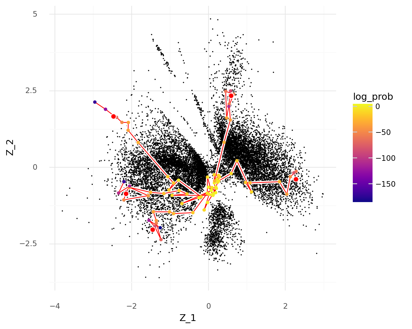
As the $ \texttt{log_prob}_c $ term decreases, cells are more likely to be represented inside the prior $ \text{N}(\mathbf{0}, \mathbf{1}) $.

The thinned cells can be used to visualize how the relation between the $ \texttt{log_prob}_c $ term and the $ \mathtt{kl}_c $ term depend on the total UMI count depth $ \ell_c $.

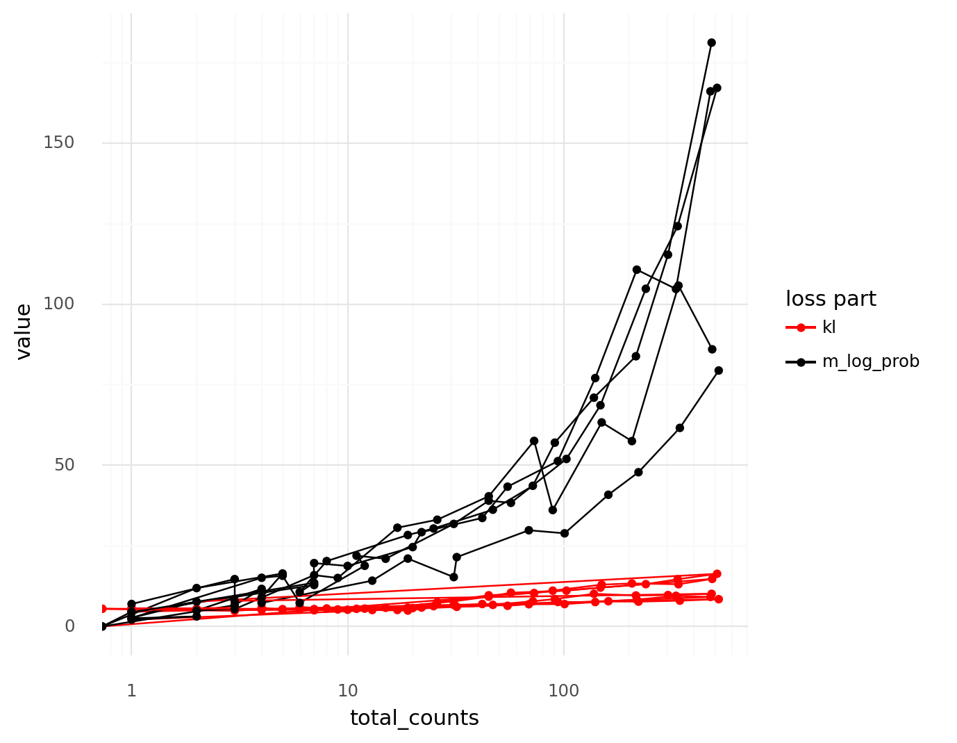
Below a threshold, the magnitude of the $ -\texttt{log_prob}_c $ term is of the same magnitude as the $ \texttt{kl}_c $ term.

This explains the phenomenon of lower quality cells with fewer UMI counts landing in the center of the latent scVI representation. The intuition to keep in mind is that for count distributions, when you count fewer items you have less information than when you count more items. In these cases, information from the prior is used instead, which constrains the representations to the center.

This also highlights the value of obtaining cells with high UMI counts. If all cells in an analysis have extremely low UMI counts, it will be hard to escape the prior to learn cell states (which manifest as dense regions of the latent representation space). When working with cells that have low UMI counts, be comfortable with their identities being ambiguous; you simply can’t learn as much from them as cells with higher counts.

Notebooks for the analysis in this post are available on Github at https://github.com/vals/Blog/tree/master/230524-center-of-scvi-space.

Ren, Xianwen, Wen Wen, Xiaoying Fan, Wenhong Hou, Bin Su, Pengfei Cai, Jiesheng Li, et al. 2021. “COVID-19 Immune Features Revealed by a Large-Scale Single-Cell Transcriptome Atlas.” Cell 184 (23): 5838. https://doi.org/10.1016/j.cell.2021.10.023.