ZINB-WaVE in Stan for scRNA-seq analysis — What do you mean "heterogeneity"?

Recently Risso et al published a paper where they define a pretty much complete model for single cell RNA-sequencing. It has all the components you would want, and addresses pretty much all problems you get asked about when giving scRNA-seq talks.

The model is called ZINB-WaVE (Zero-Inflated Negative Binomial-based Wanted Variation Extraction), and if you have and expression matrix \( y \) of \( I \) cells and \( J \) genes written out in its complete form, it looks like this

\[ \begin{align} \text{ZINB}(y_{i, j} | \mu_{i, j}, \theta_{i, j}, \pi_{i, j}) &= \pi_{i, j} \cdot \delta_0(y_{i, j}) - (1 - \pi_{i, j}) \cdot \text{NB}(y_{i, j} | \pi_{i, j}, \theta_{i, j}) \\ \ln(\mu_{i, j}) &= (X \beta_\mu + (V \gamma_\mu)^\top + W \alpha_\mu + O_\mu)_{i, j} \\ \text{logit}(\pi_{i, j}) &= (X \beta_\pi + (V \gamma_\pi)^\top + W \alpha_\pi + O_\pi)_{i, j} \\ \ln(\theta_{i, j}) &= \zeta_j \end{align} \]

This model handles over-dispersed count noise by using the negative binomial likelihood. It handles the dropouts in scRNA-seq data by making a zero-inflated version of the likelihood. The expression level (\( \mu \)) and dropout probability (\( \pi \)) are both modeled by linear regression. The factor \( X \beta \) is linear regression based on known sample covariates. This means you can directly include a term for e.g. batches or cDNA quality. Similarly, the \( V \gamma \) term is a regression with known gene covariates, which means you can include information about e.g. gene length or GC content to mitigate amplification biases.

Now, the \(W \alpha \) factor is a latent decomposition of the remaining variance after the two regression models. Similarly to what I wrote about in the RCA post, we need to learn both the entries in \(W \) and \( \alpha \). (I haven't understood the point of the offset matrices \( O \)). If we pre-determine \( W \) to have 2 columns, we will find a 2D representation of the data while also correcting for all the different biases which causes issues with standard methods such as PCA.

In particular, my facourite part of this model is that by requiring intercept terms to be part of both \( X \) and \(V \), the expression levels of different genes will be automatically normalised to the fact that different cells have different sequencing library sizes. There's a huge number of cross-sample normalisation strategies for this kind of data, any of which further need to be variance-stabalised and standard scaled in order for PCA to make sense.

To me this looks nice but sounds like it would be impossible to find a good fit for. But Risso et al show in their paper that they have come up with a strategy to do the inference, and claim it runs in a few minutes for normal data sets. In particular, they select the top 1,000 genes in terms of variance when performing analysis, which help a lot with the number of parameters in the model.

Stan implementation

I wanted to try this out, so I implemented ZINB-WaVE in Stan, the full implementation looks like this:

```
data {
    int<lower=0> N; // number of data points in dataset
    int<lower=1> P; // number of known covariates
    int<lower=1> K; // number of hidden dimensions
    int<lower=1> G; // number of observed genes
    int<lower=1> C; // number of observed cells

    vector[P] x[N]; // Covariates, including intercept.
    int y[N];      // Expression values (counts!)
    int<lower=1, upper=G> gene[N]; // Gene identifiers
    int<lower=1, upper=C> cell[N]; // Cell identifiers

    }
    parameters {
    // Latent variable model
    matrix[G, K] alpha_mu;
    matrix[G, K] alpha_pi;

    matrix[K, C] w;

    // Cell regression weights
    matrix[G, P] beta_mu;
    matrix[G, P] beta_pi;

    // Gene regression weights
    // (For now only do intercept)
    matrix[G, 1] gamma_mu;
    matrix[G, 1] gamma_pi;

    // Dispersion
    real zeta[G];

    }
    model {
    row_vector[1] mu;
    row_vector[1] pi_;
    real theta;

    // Priors
    to_vector(w) ~ normal(0, 1);

    // likelihood
    for (n in 1:N){
        mu = exp(beta_mu[gene[n]] * x[n] + gamma_mu[gene[N]] + alpha_mu[gene[n]] * col(w, cell[n]));
        pi_ = beta_pi[gene[n]] * x[n] + gamma_pi[gene[N]] + alpha_pi[gene[n]] * col(w, cell[n]);
        theta = exp(zeta[gene[n]]);

        if (y[n] > 0) {
            target += bernoulli_logit_lpmf(0 | pi_) + neg_binomial_2_lpmf(y[n] | mu, theta);
        }
        else {
            target += log_sum_exp(bernoulli_logit_lpmf(1 | pi_),
                                    bernoulli_logit_lpmf(0 | pi_) + neg_binomial_2_lpmf(y[n] | mu, theta));
        }
    }
}
```

Here I'm using a long-form ("tidy") representation of the data, but the likelihood is just essentially what I wrote in the equation above. It took me a while to get the zero-inflation working correctly, but the rest was pretty straight forward. I didn't include the per-gene covariates beyond the intercept for normalisation.

Application to stem cell data

I grabbed some data from Velten et al which I had previously processed using our umis tool for our methods comparison.

The consists of single-cell RNA-seq UMI counts using the BATSeq method. They sequenced mESC's from different culture conditions (Serum and 2i), as well as NSC's.

I performed some quick quality assessment of the data by investigating the relation between the number of genes with at least one count, and the total UMI count in a given cell for all genes.

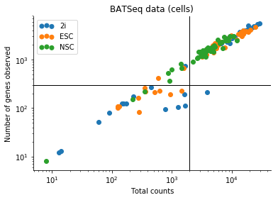
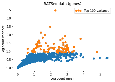
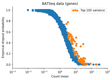
Based on this I filtered the samples based on some thresholds, and picked out the 100 genes which had the highest log count variance. (Stan is not as fast as Risso et al's implementation, 1,000 genes takes too long to run for my taste).

The Velten et al data contains reads from ERCC spike-ins. We might observe variation in the data which is due only to differences in relative spike-in abundance. Cells with more RNA will have less reads assigned to spike-ins, so globally, this will affect expression of all genes in a non-interesting sense. To retain interesting variation in the data, we can use the \( X \beta \) factor to account for variation due to ERCC content. So one columns of \( X \) is \( 1 \) (intercept), and the second column of \( X \) will be log(ERCC counts) for each cell.

After a slightly messy data-conversion to the long-form format I made the Stan model for, I ran ADVI for the data until convergence (~2,500 iterations) which took a minute or two. The quantities we are interested in are the two columns of \(W \) which represent variation in the data.

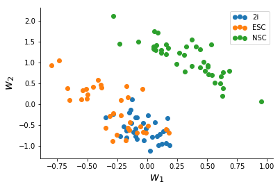
We note that NSC's seperate clearly from mESC's, and based on this there might be more heterogeneity in Serum mESC's than 2i mESC's.

Notebook of the analysis available here.

Extensions

So what can we use this for? The Stan implementation is slower and less immidiately user-friendly than the R package by Risso et al. However, the Stan model provides us with a sort of canvas which can be used to prototype variations of this model. Just editing a few lines, we can compare the results of ZINB-WaVE with e.g. results from using the drop-out model in ZIFA.

Something I'm interested in is whether the model can be extended to get a notion of "% variance explained" from the \( W \) factors using Automatic Relevence Determination. I'm not completely sure, but I think this means making the model hierarchical with \[ \log(\mu) \sim \mathcal{N}(X \beta_\mu + (V \gamma_\mu)^\top + W \alpha_\mu + O_\mu, \sigma^2) \] and then put priors on the columns of \( W \).