Explaining variance by technical factors in scRNA-seq data using ARD-MLR in Stan

I was recently rereading the ADVI paper by Kucukelbir et al and noted a couple of things I didn't know. First of all, their Stan implementation of Probabilistc PCA (PPCA) in the paper is far better than the implementation I made. Secondly, they implement a version of PPCA with Automatic Relevence Determination (ARD). This gives the ability to extract "fraction variance explained" of the principal components similar to the Singular Value Decomposition based implementatoins.

In PPCA we seek matrices W and Z so that

\(\begin{align} X_n & \sim \mathcal{N}(W \cdot Z_n + \mu, \sigma^2), \\ Z_{i,j} & \sim \mathcal{N}(0, 1), \\ W_{i,j} & \sim \mathcal{N}(0, \sigma^2). \end{align}\)

The modification that allows the ARD is to introduce a hyper-prior α for the prior on the weights W.

\(W_{i,j} \sim \mathcal{N}(0, \alpha_j \cdot \sigma^2).\)

Now the posterior of α will indicate the proportion of variation of a given column of Z explains the variance of X.

This seem to work really nicely, and applies directly to the Residual Component Analysis model I described in an earlier post.

This idea of putting the hyper-prior on the variance solve another thing I've been trying to do though, which I'll describe below.

When I get a new single-cell RNA-seq dataset, I usually try to figure out what known factors are contributing to variation in the data. We usually have a table with technical and experimental information, as well as a gene expression matrix for each gene in each sample.

For now the RCA is really too slow to be applicable to scRNA-seq data. My general workflow goes like this:

1. Perform PCA

2. Correlate PCs with technical factors

3. Regress out correlating technical factors

4. Perform PCA on the residuals

5. Repeat step 2-4 until you understand the data for proper analysis

This gives me a handle on which factors are responsible to alot of variation, and various average effect sizes and groupings. It does not however give me quantitative information about how much of the variation in the data is explained by the different factors! I've been a bit frustrated with this since the PC's do come with this information, so I've felt it should be possible to get this information in a supervised way. I know it something which can be done, but I haven't found the correct Google terms, which I guess should be something like "variance explained in multivariate multiple linear regression".

In the ARD-PPCA model above though, I saw a clear strategy to get the values I want to know. Perform Multiple Linear Regression with an ARD hyper-prior!

I made a Stan implementation which takes multivariate data and a design matrix assumed to include an intercept.

data {
  int<lower=0> N; // number of data points in dataset
  int<lower=0> D; // dimension

  int<lower=0> P; // number of known covariates
  vector[D] x[N]; // data
  matrix[P, N] y; // Knwon covariates

}
parameters {
  real<lower=0> sigma;
  matrix[D, P] w_y;
  vector<lower=0>[P] beta;
}
model {
  // priors
  for (d in 1:D){
    w_y[d] ~ normal(0, sigma * beta);
  }
  sigma ~ lognormal(0, 1);
  beta ~ inv_gamma(1, 1);

  // likelihood
  for (n in 1:N){
    x[n] ~ normal (w_y * col(y, n), sigma);
  }
}

Then I grabbed a data set I had lying around (with 96 samples). Below is a snipped of the kind of sample information available.

21681_1#18 21681_1#32 21681_1#48 21681_1#58 21681_1#12 detection_limit inf inf inf inf inf accuracy -inf -inf -inf -inf -inf ERCC_content 0 0 0 0 0 num_genes 7092 6990 469 6056 1025 MT_content 72193.3 82527.8 77319.3 97045.6 99507.8 rRNA_content 68.1274 41.7641 1905.97 41.2784 0 num_processed 680970 7287104 975356 3726116 27173 num_mapped 501237 6106642 670644 3081850 2018 percent_mapped 73.6063 83.8007 68.7589 82.7094 7.42649 global_fl_mode 321 1000 309 276 283 robust_fl_mode 321 280 309 276 283 Supplier Sample Name SCGC--0894_B06 SCGC--0894_C08 SCGC--0894_D12 SCGC--0894_E10 SCGC--0894_A12 sample_type sc sc sc sc sc LB_type A B B B B merge sc_A sc_B sc_B sc_B sc_B well B06 C08 D12 E10 A12 row 2 3 4 5 1 column 6 8 12 10 12

Using the patsy Python package, we can generate a design matrix which we use to model the values in the expression matrix.

Y = patsy.dmatrix('np.log(num_genes) + np.log(num_mapped) + LB_type + sample_type + percent_mapped', sample_info, return_type='dataframe')

While the ADVI in Stan is fast, I didn't have the patiance to run the model on the full expression matrix. In stead I sampled 1,000 genes and ran the model on that, just as a prookf of concept.

partial_logexp = logexp.sample(1000, axis=0)

N, D = partial_logexp.T.shape
N, P = y.shape
data = {
    'N': N,
    'D': D,
    'x': partial_logexp.T,
    'P': P,
    'y': y.T
}

v = model.vb(data=data)

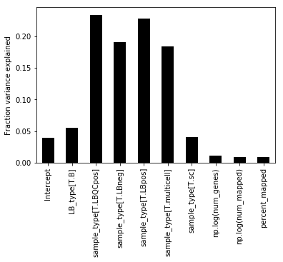
As you might see from the Stan code, the ARD parameter is β, so we extract these for the different columns of the design matrix Y.

Note that the one-hot encoding for the categorical variables is spreading variance in to multiple columns. To get a final fraction we can sum over all the variance for a given categorical variable.

We see that the majority of variance in the data is due to sample_type, which indicate whether a sample is proper, or positive control or negative control. After this the LB_type parameter explains the second most amount of variance. (Which is a sample condition for this data, but it's not very important exactly what it is in the proof of concept).

It seems pretty stable for sub-samples of genes during my experimentation. I think this might be a neat way to quickly assess your data. I'm not sure how fast it will run for more samples though, even when sampling only 1,000 genes.

A notebook of this can be found here.

I really like how quickly problems can be solved, at least to the prototype stage, using probabilistic programming like with Stan. This short model solves a problem in an intuitive way. And the conciseness of the language meant I could write the entire model on the bus home from work.